Perhaps the most commonly used datasets from Brazilian censuses are
the microdata of individuals and households. Nonetheless, IBGE also
makes available some extremely data on population and environmental
characteristics aggregated at the census tract level. In this vignette,
we show how to use the {censobr} package to easily
access census tract-level data using the read_tracts()
function.
At the moment, this function includes data from the censuses of 2000, 2010 and 2022.
Data structure
Aggregated data at the census tract level are split into different datasets, and some of them are scattered across several files. For the sake of convenience, we have gathered all of the files into different datasets:
| 2000 | 2010 | 2022 |
|---|---|---|
| Basico | Basico | Basico |
| Domicilio | Domicilio | Domicilio |
| Pessoa | Pessoa | Pessoas |
| Responsavel | Responsavel | |
| Instrucao | Entorno | Entorno |
| Morador | ResponsavelRenda | ResponsavelRenda |
| DomicilioRenda | Indigenas | |
| PessoaRenda | Quilombolas | |
| Obitos | ||
| Preliminares |
All of the data aggregated at census tracts are organized following the same logic.
In the cases when there are multiple files in the same dataset, we
add a reference to the number of the file as a prefix to the variable
name. To illustrate this, let’s have a look at the
"Domicilio" dataset. This dataset is based on three
separate tables: Domicilio01, Domicilio02 and
Domicilio03. So the names of the columns in this dataset are
organized as follows:
library(censobr)

dom <- read_tracts(
  year = 2022,
  dataset = 'Domicilio',
  showProgress = FALSE
  )
#> ℹ Reading data cached locally.

names(dom)[c(30:33,119:121, 526:528)]
#>  [1] "CD_SETOR"           "CD_SIT"             "CD_TIPO"
#>  [4] "CD_REGIAO"          "domicilio01_V00063" "domicilio01_V00064"
#>  [7] "domicilio01_V00065" "domicilio02_V00470" "domicilio02_V00471"
#> [10] "domicilio02_V00472"
Dictionary of variables
To check the meaning of each variable, users can run the
data_dictionary(), which returns the path to the file with
the dictionary of variables, and opens it in an interactive session. The
dictionary file is either a .pdf or an .xlsx
file, depending on the data set and year.
data_dictionary(
  year = 2022,
  dataset = 'tracts'
  )
Reproducible examples
Now let’s use a couple reproducible examples to illustrate how to work with census tract-level data. First, we need to load the libraries we’ll be using in this vignette.
In these examples below, example we’ll use the city of Belo Horizonte for demonstration purposes. So we can start by downloading the the geometries of the census tracts in the area. First, we need to download the geometries of all census tracts in the state of Minas Gerais (MG), and then keep only the ones in the municipality of Belo Horizonte. We’ll also download the municipality borders of BH.
muni_bh <- geobr::read_municipality(
  code_muni = 'MG',
  year = 2010,
  showProgress = FALSE
  ) |>
  filter(name_muni == "Belo Horizonte")
#> ℹ Using year/date 2010
#> duckdb keeps downloaded extensions and secrets in a temporary directory:
#> ℹ /tmp/RtmpEn8ysU/duckdb
#> This is removed when the R session ends.
#> • Extensions are re-downloaded each session.
#> • Secrets are lost.
#> ℹ Run duckdb(shared_home = TRUE) (or create ~/.duckdb) to keep them (suitable for most users).
#> ℹ Run duckdb(shared_home = FALSE) to accept the temporary directory (and silence this message).
#> ℹ See ?duckdb_storage for details and alternatives.

tracts_sf <- geobr::read_census_tract(
  code_tract = "MG",
  simplified = FALSE,
  year = 2010,
  showProgress = FALSE
  )
#> ℹ Using year/date 2010

tracts_sf <- filter(tracts_sf, name_muni == "Belo Horizonte")

ggplot() +
  geom_sf(data = tracts_sf, fill = 'gray90', color = 'gray60') +
  theme_void()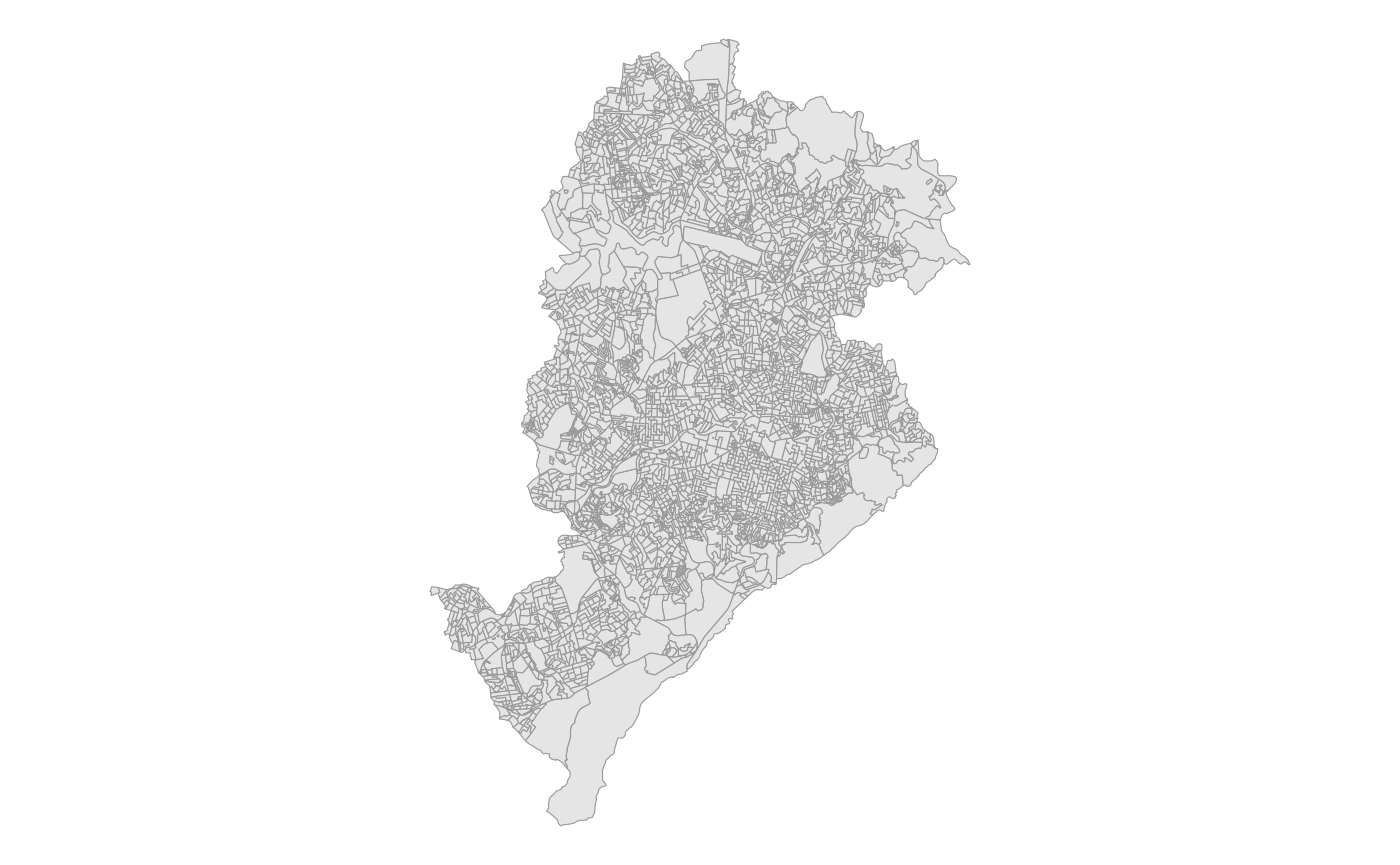
Example 1:
In this first example we are going to map the proportion of
households with the presence of trees in their surroundings. To do this,
we need to download the "Entorno" dataset and sum the
variables
domicilios_V05031 + domicilios_V05032 + domicilios_V05033.
# download data
tract_entorno <- censobr::read_tracts(
  year = 2022,
  dataset = "Entorno",
  showProgress = FALSE
  )
#> ℹ Downloading data and storing it locally for future use.

# filter observations and calculate indicator
df_trees <- tract_entorno |>
  filter(code_tract %in% tracts_sf$code_tract) |>
  group_by(code_tract) |>
  mutate(total_households = domicilios_V05000,
         trees = domicilios_V05031 + domicilios_V05032+ domicilios_V05033,
         trees_prop = trees / total_households) |>
  select(code_tract, total_households, trees, trees_prop) |>
  collect()

head(df_trees)
#> # A tibble: 6 × 4
#> # Groups:   code_tract [6]
#>   code_tract total_households trees trees_prop
#>        <dbl>            <int> <int>      <dbl>
#> 1    3.11e14              222   222      1
#> 2    3.11e14              158   158      1
#> 3    3.11e14              294   294      1
#> 4    3.11e14              131   131      1
#> 5    3.11e14              142   138      0.972
#> 6    3.11e14              218   218      1
Now we can merge the spatial data with our indicator and see how the presence of trees in the surroundings of households varies spatially.
bh_tracts <- left_join(tracts_sf, df_trees, by = 'code_tract')

ggplot() +
  geom_sf(data = bh_tracts, aes(fill = trees_prop), color=NA) +
  geom_sf(data = muni_bh, color='gray10', fill=NA) +
  labs(subtitle = 'Share of households with trees in their surroundings.\nBelo Horizonte, 2010') +
  scale_fill_distiller(palette = "Greens", direction = 1,
                       name='Share of\nhouseholds',
                       na.value = "gray90",
                       labels = scales::percent) +
  theme_void()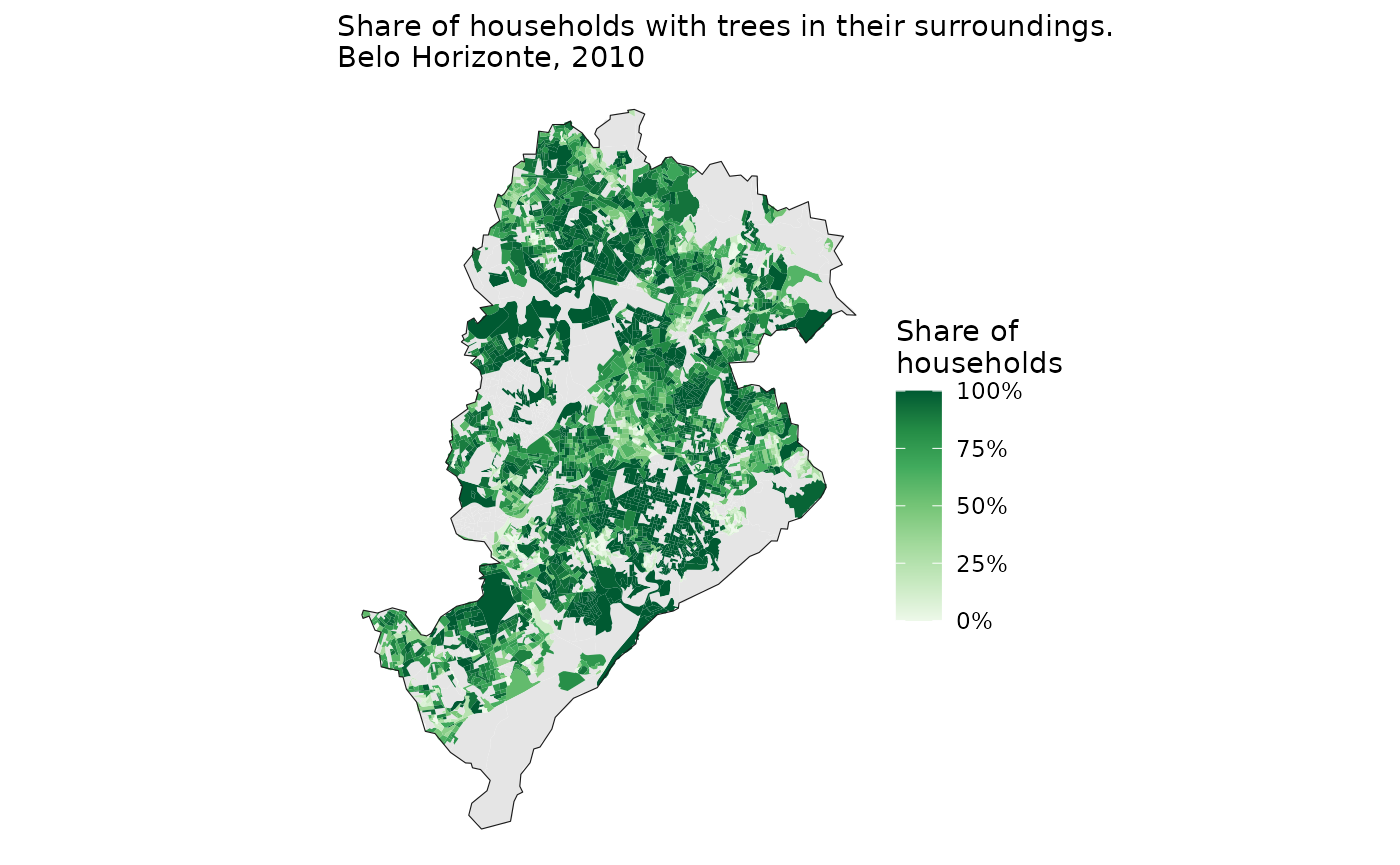
Example 2: Spatial distribution of income
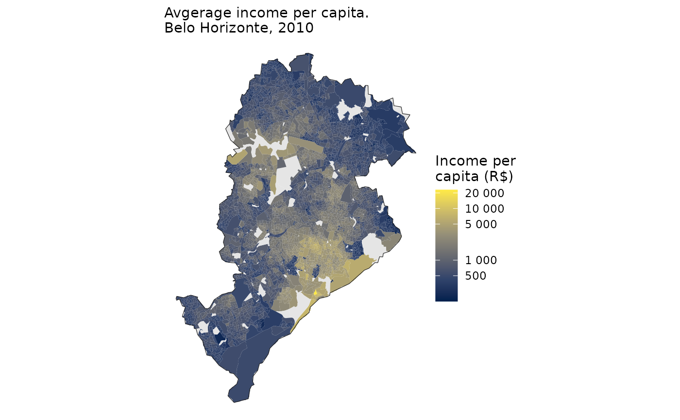
In this second example, we are going to create a map of the spatial distribution of average income per capita. Unfortunately, this information was not collected in the 2022 census at the census tract level, so this example is based on the 2010 data.
In the 2010 census, we can find the information on the the total
number of residents in each census tract in the "Basico"
dataset, variable "V002". Meanwhile, the information on
income can be found in the "DomicilioRenda" dataset,
variable "V003".
Using the code below, we download the data and calculate the income per capita of all census tracts in Brazil.
# download data
tract_basico <- censobr::read_tracts(
  year = 2010,
  dataset = "Basico",
  showProgress = FALSE
  )
#> ℹ Reading data cached locally.

tract_income <- censobr::read_tracts(
  year = 2010,
  dataset = "DomicilioRenda",
  showProgress = FALSE
  )
#> ℹ Downloading data and storing it locally for future use.

# select columns
tract_basico <- tract_basico |> select('code_tract','V002')
tract_income <- tract_income |> select('code_tract','V003')

# merge
tracts_df <- left_join(tract_basico, tract_income) |> collect()

# calculate income per capita
tracts_df <- tracts_df |> mutate(income_pc = V003 / V002)
head(tracts_df)
#> # A tibble: 6 × 4
#>   code_tract  V002   V003 income_pc
#>        <dbl> <int>  <int>     <dbl>
#> 1    1.10e14   956 522231      546.
#> 2    1.10e14   859 406191      473.
#> 3    1.10e14   661 241587      365.
#> 4    1.10e14   266  88502      333.
#> 5    1.10e14  1206 262860      218.
#> 6    1.10e14   816 262968      322.
Finally, we can merge the spatial data with our per capita income estimates and map the results.
bh_tracts <- left_join(tracts_sf, tracts_df, by = 'code_tract')

ggplot() +
  geom_sf(data = bh_tracts, aes(fill = income_pc), color=NA) +
  geom_sf(data = muni_bh, color='gray10', fill=NA) +
  labs(subtitle = 'Avgerage income per capita.\nBelo Horizonte, 2010') +
  scale_fill_viridis_c(name = "Income per\ncapita (R$)",
                       labels = scales::number_format(),
                       option = 'cividis',
                       breaks = c(0, 500, 1e3, 5e3, 1e4, 2e4),
                       trans = "pseudo_log", na.value = "gray90") +
  theme_void()