The geobr package provides quick and easy access to official spatial data sets of Brazil. The package offers a wide range of spatial data sets available at various geographic scales and for various years with harmonized attributes, projection and fixed topology. All geobr functions follow a simple and consistent syntax that allows users to seamlessly download data and work with it either in memory using GeoPandas or out of memory using DuckDB and Arrow. This vignette presents a quick intro to geobr.
Installation
You can install geobr from PyPI:
pip install geobr
Now let’s load the libraries we’ll use in this vignette.
General usage
Available data sets
The geobr package currently covers 30 spatial data sets, including a
variety of political-administrative and statistical areas used in
Brazil. You can view what data sets are available using the
list_geobr() function.
| Function | geography | source | alias | years_available | |
|---|---|---|---|---|---|
| 0 | read_country | Country | IBGE | country | 1872, 1900, 1911, 1920, 1933, 1940, 1950, 1960, 1970, 1980, 1991, 2000, 2001, 2010, 2013, 2014, 2015, 2016, 2017, 2018, 2019, 2020, 2021, 2022, 2023, 2024, 2025 |
| 1 | read_region | Region | IBGE | regions | 1872, 1900, 1911, 1920, 1933, 1940, 1950, 1960, 1970, 1980, 1991, 2000, 2001, 2010, 2013, 2014, 2015, 2016, 2017, 2018, 2019, 2020, 2021, 2022, 2023, 2024, 2025 |
| 2 | read_state | States | IBGE | states | 1872, 1900, 1911, 1920, 1933, 1940, 1950, 1960, 1970, 1980, 1991, 2000, 2001, 2010, 2013, 2014, 2015, 2016, 2017, 2018, 2019, 2020, 2021, 2022, 2023, 2024, 2025 |
| 3 | read_meso_region | Meso region | IBGE | mesoregions | 2000, 2001, 2013, 2014, 2015, 2016, 2017, 2018, 2019, 2020, 2021, 2022 |
| 4 | read_micro_region | Micro region | IBGE | microregions | 2000, 2001, 2013, 2014, 2015, 2016, 2017, 2018, 2019, 2020, 2021, 2022 |
Download spatial data as GeoDataFrames
The syntax of all geobr functions operate on the same logic, so the code to download the data becomes intuitive for the user. Here are a few examples.
Download a specific geographic area at a given year
# State of Sergige
state = geobr.read_state(code_state="SE", year=2018)
# Municipality of Sao Paulo
muni = geobr.read_municipality(code_muni=3550308, year=2010)
Download all geographic areas within a state at a given year
# All municipalities in the state of Alagoas
muni = geobr.read_municipality(code_muni="AL", year=2007)

# All census tracts in the state of Rio de Janeiro
cntr = geobr.read_census_tract(code_tract="RJ", year=2010)
If the parameter code_ is not passed to the function,
geobr returns the data for the whole country by default.
Important note about data resolution
All functions to download polygon data such as states, municipalities
etc. have a simplified argument. When
simplified=False, geobr will return the original data set
with high resolution at detailed geographic scale (see documentation).
By default, however, simplified=True and geobr returns data
set geometries with simplified borders to improve speed of downloading
and plotting the data.
Plot the data
Once you’ve downloaded the data, it is really simple to plot maps
using matplotlib.
# Plot all Brazilian states
fig, ax = plt.subplots(figsize=(15, 15), dpi=300)

states.plot(facecolor="#2D3E50", edgecolor="#FEBF57", ax=ax)

ax.set_title("States", fontsize=20)
ax.axis("off")
(-76.24758052685, -26.590708254149995, -35.70232894755864, 7.22299203073151)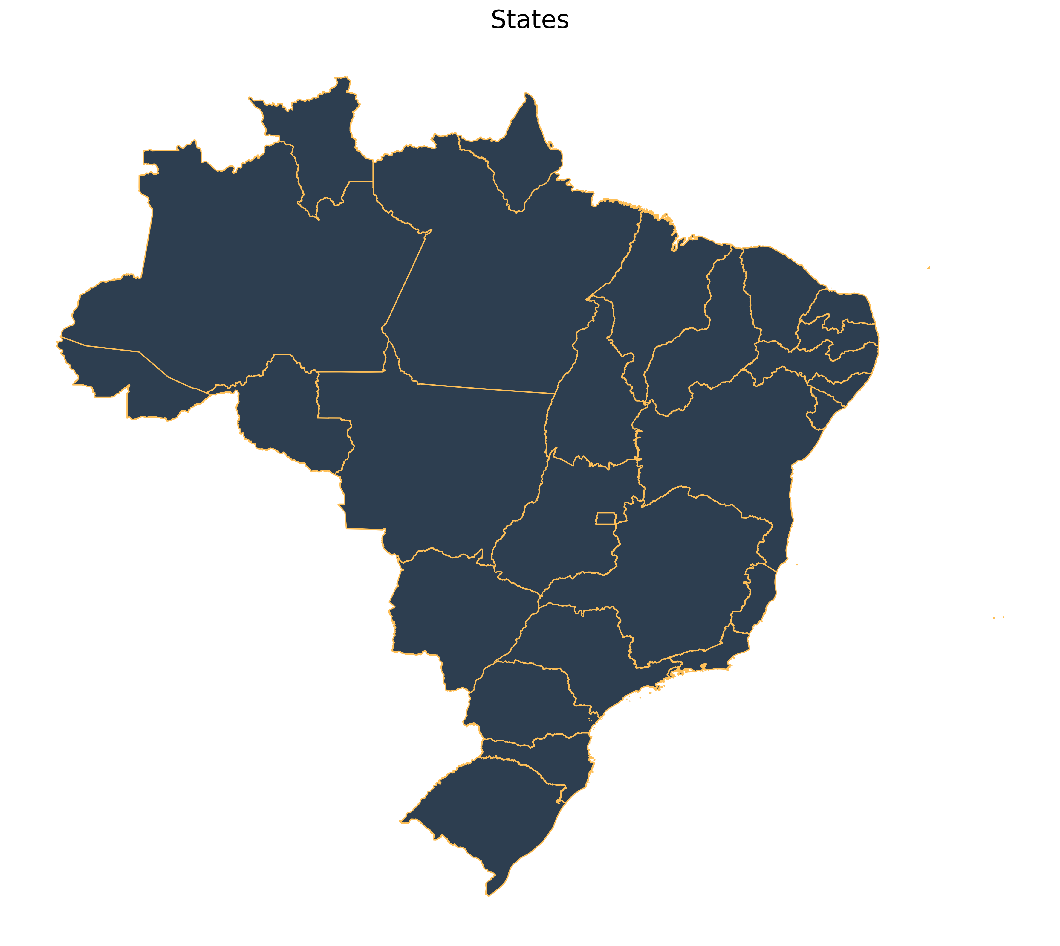
Plot all the municipalities of a particular state, such as Rio de Janeiro:
# plot
fig, ax = plt.subplots(figsize=(15, 15), dpi=300)

all_muni.plot(facecolor="#2D3E50", edgecolor="#FEBF57", ax=ax)

ax.set_title("Municipalities of Rio de Janeiro, 2000", fontsize=20)
ax.axis("off")
(-45.08586065211478,
-40.7619784166046,
-23.499218287945578,
-20.632919136978526)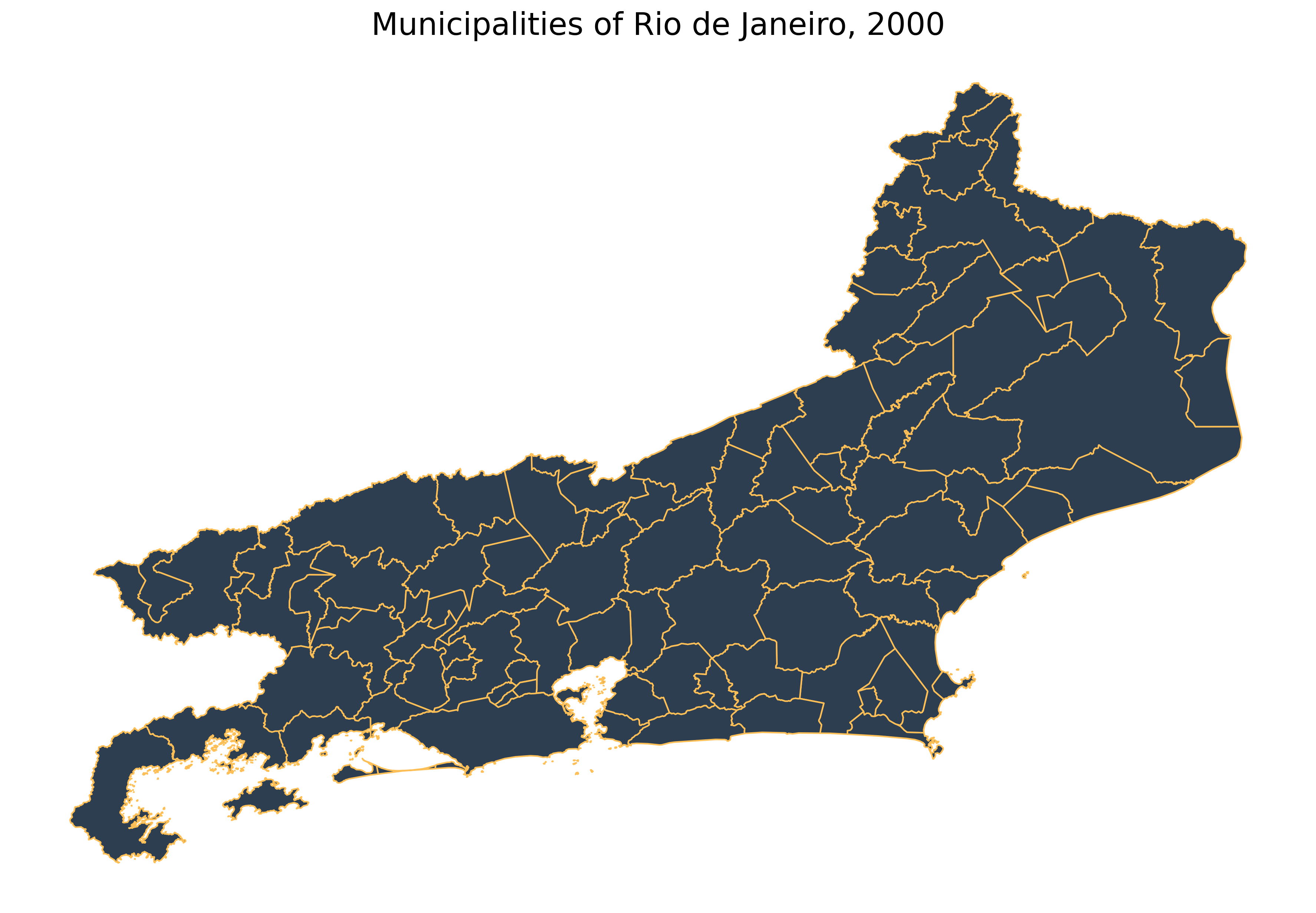
Lazy evaluation with DuckDB and Arrow
By default, all functions in geobr use output = "gpd"
and return a GeoPandas’ geodataframe object loaded into
memory. In some cases, however, it may be preferable to process data out
of memory for faster and more memory-efficient computation, particularly
when working with large spatial data sets.
To support these workflows, users can set
output = "duckdb" to return a lazy
DuckDBPyRelation object. It uses the official DuckDB
Spatial extansion to enable a “GEOMETRY” data type. This allows data to
be analyzed with DuckDB, enabling efficient out-of-memory spatial
operations. Users can also leverage a DuckDB power-user API with
auto-resolving query(), as shown in this example.
Alternatively, users can set output = "arrow" to return
an Arrow dataset, which can be integrated with the Arrow ecosystem for
scalable analytical workflows. Note that PyArrow lacks a special
geometry data type and does not natively process geographic coordinates
without extra tools. Geobr returns the geometry column
stored as Well-Known Binary (WKB) byte arrays and the user can use the
GeoArrow library for optimized spatial operations.
Thematic maps
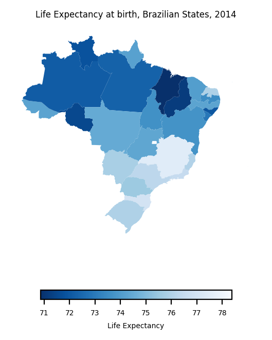
The next step is to combine data from geobr package with other data sets to create thematic maps. In this example, we will be using data from the (Atlas of Human Development (a project of our colleagues at Ipea) to create a choropleth map showing the spatial variation of Life Expectancy at birth across Brazilian states.
Merge external data
First, we need a DataFrame with estimates of Life
Expectancy and merge it to our spatial database. The two-digit
abbreviation of state name is our key column to join these two
databases.
# Read DataFrame with life expectancy data
data_url = "https://raw.githubusercontent.com/ipea/geobr/master/r-package/inst/extdata/br_states_lifexpect2017.csv"

df = pd.read_csv(data_url, index_col=0)

states["name_state"] = states["name_state"].str.lower()
df["uf"] = df["uf"].str.lower()

# join the databases
states = states.merge(df, how="left", left_on="name_state", right_on="uf")
Plot thematic map
plt.rcParams.update({"font.size": 5})

fig, ax = plt.subplots(figsize=(4, 4), dpi=200)

states.plot(
    column="ESPVIDA2017",
    cmap="Blues_r",
    legend=True,
    legend_kwds={
        "label": "Life Expectancy",
        "orientation": "horizontal",
        "shrink": 0.6,
    },
    ax=ax,
)

ax.set_title("Life Expectancy at birth, Brazilian States, 2014")
ax.axis("off")
(-76.24758052684999,
-26.590708254149995,
-35.70232894755864,
7.222992030731511)