
Abstract
This vignette shows how to calculate and visualize accessibility in R using ther5r package.
1. Introduction
Accessibility indicators measure how easily opportunities, such as
jobs, can be reached from a given location (Levinson and et al. 2020). This vignette
calculates and maps accessibility with the r5r
package, using the Porto Alegre (Brazil) sample data included in
r5r, in two ways:
-
quick:
r5r::accessibility(); -
flexible: an
r5rtravel time matrix passed to the {accessibility} package, which offers a wider range of metrics.
2. Build routable transport network with
build_network()
Increase Java memory and load libraries
Set Java memory before loading the packages (why).
options(java.parameters = "-Xmx2G")

library(r5r)
library(accessibility)
library(sf)
library(data.table)
library(ggplot2)
library(interp)
library(h3jsr)
library(dplyr)
build_network() takes the directory holding the
OpenStreetMap and GTFS data:
# system.file returns the directory with example data inside the r5r package
# set data path to directory containing your own data if not running this example
data_path <- system.file("extdata/poa", package = "r5r")

r5r_network <- build_network(data_path)
3. Accessibility: quick and easy approach
One of the simplest accessibility metrics is the
cumulative-opportunity metric: the number of opportunities reachable
within a travel time cutoff (decay_function = "step").
Here we count the schools (points$schools) and public
healthcare facilities (points$healthcare) reachable by
public transport in less than 20 minutes, using the median travel time
of departures every minute over a 60-minute window (2pm to 3pm).
accessibility() handles several opportunity types in one
call, which is much more efficient than computing a travel time matrix
and aggregating it yourself.
# read all points in the city
points <- fread(file.path(data_path, "poa_hexgrid.csv"))

# routing inputs
mode <- c("WALK", "TRANSIT")
max_walk_time <- 30      # in minutes
travel_time_cutoff <- 20 # in minutes
time_window <- 60        # in minutes
departure_datetime <- as.POSIXct("13-05-2019 14:00:00",
                                 format = "%d-%m-%Y %H:%M:%S")

# calculate accessibility
access1 <- r5r::accessibility(
  r5r_network,
  origins = points,
  destinations = points,
  mode = mode,
  opportunities_colnames = c("schools", "healthcare"),
  decay_function = "step",
  cutoffs = travel_time_cutoff,
  departure_datetime = departure_datetime,
  max_walk_time = max_walk_time,
  time_window = time_window,
  progress = FALSE
  )

head(access1)
#>                 id opportunity percentile cutoff accessibility
#>             <char>      <char>      <int>  <int>         <num>
#> 1: 89a901291abffff     schools         50     20             3
#> 2: 89a901291abffff  healthcare         50     20             5
#> 3: 89a9012a3cfffff     schools         50     20             0
#> 4: 89a9012a3cfffff  healthcare         50     20             0
#> 5: 89a901295b7ffff     schools         50     20             6
#> 6: 89a901295b7ffff  healthcare         50     20             4
r5r::accessibility() also computes gravity-based
metrics: set decay_function to "exponential",
"fixed_exponential", "linear" or
"logistic". Metrics not implemented in R5, such as floating
catchment area, travel cost to the closest N opportunities or
time-interval cumulative opportunities, are available in the
accessibility package.
4. Accessibility: flexible approach
The accessibility package takes a travel
time matrix, which we compute with r5r:
# calculate travel time matrix
ttm <- r5r::travel_time_matrix(
  r5r_network,
  origins = points,
  destinations = points,
  mode = mode,
  departure_datetime = departure_datetime,
  max_walk_time = max_walk_time,
  time_window = time_window,
  progress = FALSE
  )

head(ttm)
#>            from_id           to_id travel_time_p50
#>             <char>          <char>           <int>
#> 1: 89a901291abffff 89a901291abffff               2
#> 2: 89a901291abffff 89a9012a3cfffff              78
#> 3: 89a901291abffff 89a901295b7ffff              45
#> 4: 89a901291abffff 89a901284a3ffff              60
#> 5: 89a901291abffff 89a9012809bffff              47
#> 6: 89a901291abffff 89a901285cfffff              38
accessibility::cumulative_cutoff() computes the same
cumulative metric from the travel time matrix and land use data. It also
counts trips that take exactly the cutoff time, while
r5r::accessibility() counts only trips strictly shorter
than it, so the two estimates can differ slightly:
# calculate accessibility
access_edu <- accessibility::cumulative_cutoff(
  travel_matrix = ttm,
  land_use_data = points,
  opportunity = 'schools',
  travel_cost = 'travel_time_p50',
  cutoff = 20
  )

access_health <- accessibility::cumulative_cutoff(
  travel_matrix = ttm,
  land_use_data = points,
  opportunity = 'healthcare',
  travel_cost = 'travel_time_p50',
  cutoff = 20
  )
#> Warning: 'land_use_data$healthcare' contains NA values, which may produce NAs
#> in the final output.

head(access_edu)
#> Key: <id>
#>                 id schools
#>             <char>   <int>
#> 1: 89a9012124fffff       1
#> 2: 89a9012126bffff       4
#> 3: 89a9012127bffff       2
#> 4: 89a90128003ffff       8
#> 5: 89a90128007ffff       5
#> 6: 89a9012800bffff       8
head(access_health)
#> Key: <id>
#>                 id healthcare
#>             <char>      <int>
#> 1: 89a9012124fffff          0
#> 2: 89a9012126bffff          1
#> 3: 89a9012127bffff          1
#> 4: 89a90128003ffff          3
#> 5: 89a90128007ffff          1
#> 6: 89a9012800bffff          3
5. Map Accessibility
Two ways to map the estimates:
5.1 Choropleth maps
Each point is the centroid of a fine-resolution H3 hexagon, so we retrieve the hexagon polygons and join the accessibility estimates to them.
# retrieve polygons of H3 spatial grid
grid <- h3jsr::cell_to_polygon(points$id, simple = FALSE)

# merge accessibility estimates
access_sf <- left_join(grid, access1, by = c('h3_address'='id'))

# plot
ggplot() +
  geom_sf(data = access_sf, aes(fill = accessibility), color= NA) +
  scale_fill_viridis_c(direction = -1, option = 'B') +
  labs(fill = "Number of\nfacilities within\n20 minutes") +
  theme_minimal() +
  theme(axis.title = element_blank()) +
  facet_wrap(~opportunity) +
  theme_void()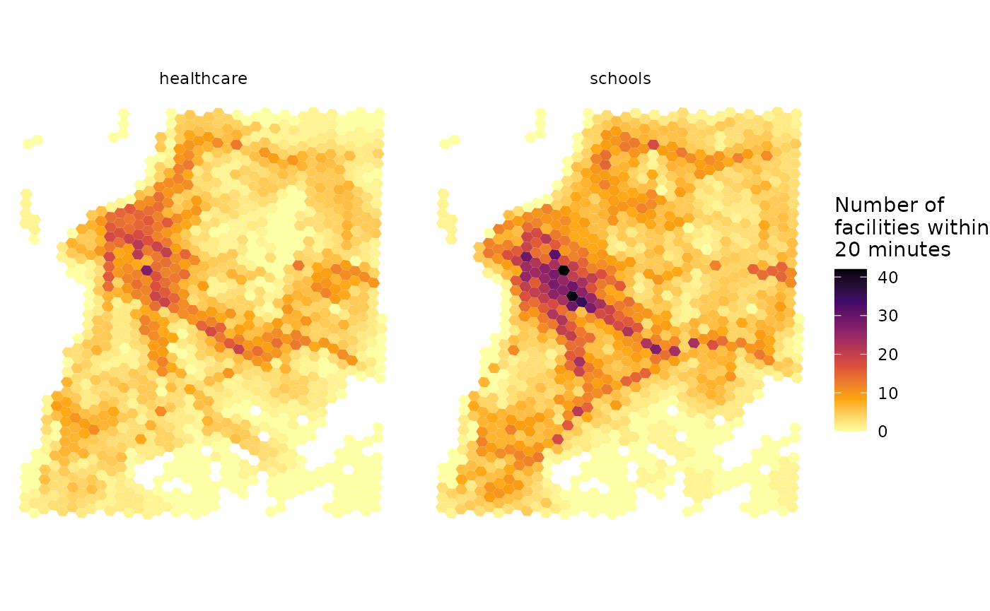
5.2 Spatial interpolation
Alternatively, interpolate the point estimates to get a smoother surface:
# interpolate estimates to get spatially smooth result
access_schools <- access1 %>%
  filter(opportunity == "schools") %>%
  inner_join(points, by='id') %>%
  with(interp::interp(lon, lat, accessibility)) %>%
  with(cbind(acc=as.vector(z),  # Column-major order
             x=rep(x, times=length(y)),
             y=rep(y, each=length(x)))) %>% as.data.frame() %>% na.omit() %>%
  mutate(opportunity = "schools")

access_health <- access1 %>%
  filter(opportunity == "healthcare") %>%
  inner_join(points, by='id') %>%
  with(interp::interp(lon, lat, accessibility)) %>%
  with(cbind(acc=as.vector(z),  # Column-major order
             x=rep(x, times=length(y)),
             y=rep(y, each=length(x)))) %>% as.data.frame() %>% na.omit() %>%
  mutate(opportunity = "healthcare")

access.interp <- rbind(access_schools, access_health)

# find results' bounding box to crop the map
bb_x <- c(min(access.interp$x), max(access.interp$x))
bb_y <- c(min(access.interp$y), max(access.interp$y))

# extract OSM network, to plot over map
street_net <- street_network_to_sf(r5r_network)

# plot
ggplot(na.omit(access.interp)) +
  geom_sf(data = street_net$edges, color = "gray55", size=0.01, alpha = 0.7) +
  geom_contour_filled(aes(x=x, y=y, z=acc), alpha=.7) +
  scale_fill_viridis_d(direction = -1, option = 'B') +
  scale_x_continuous(expand=c(0,0)) +
  scale_y_continuous(expand=c(0,0)) +
  coord_sf(xlim = bb_x, ylim = bb_y, datum = NA) +
  labs(fill = "Number of\nfacilities within\n20 minutes") +
  theme_void() +
  facet_wrap(~opportunity)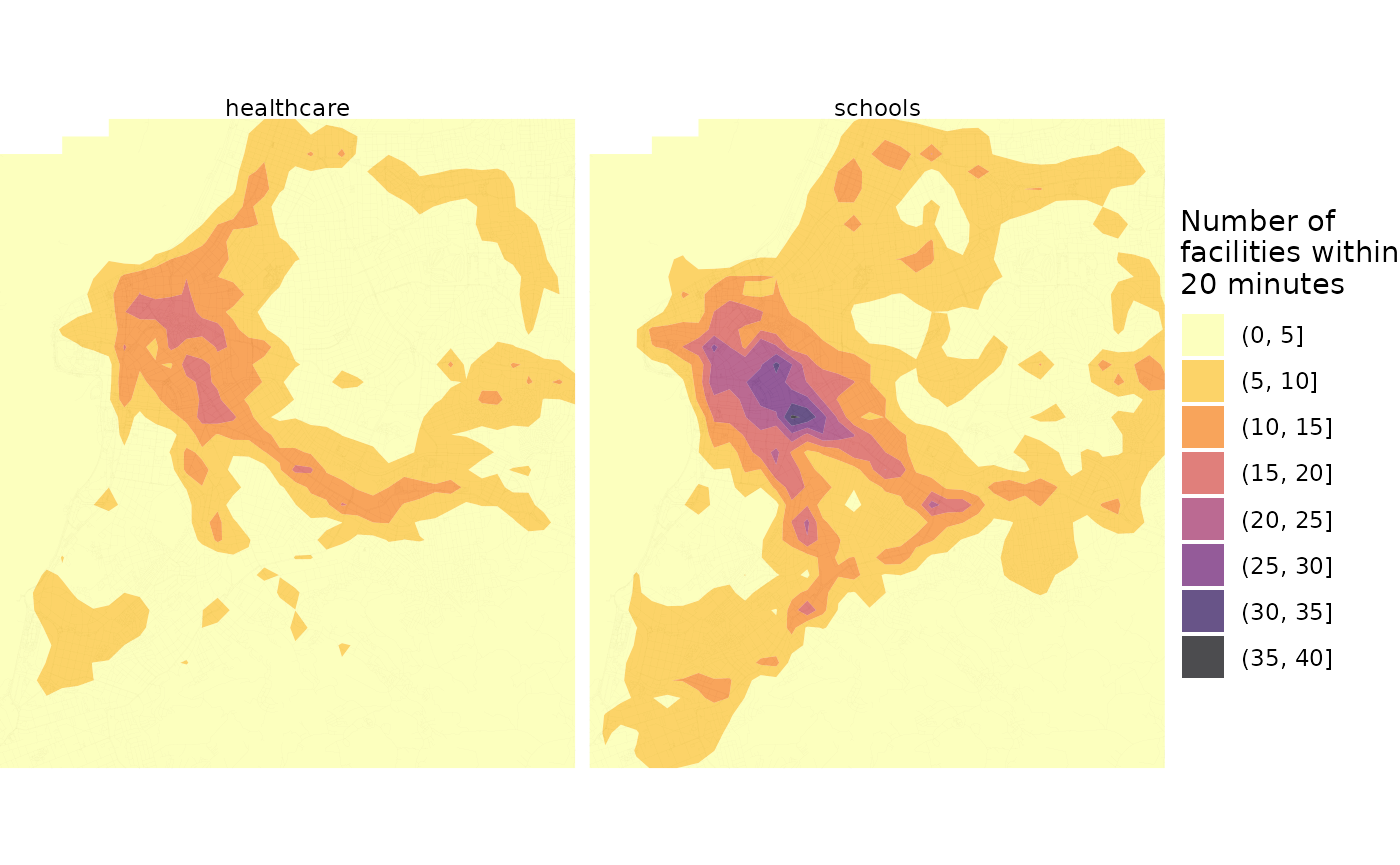
Cleaning up after usage
Stop the network and run Java’s garbage collector to free the memory it used:
If you have any suggestions or want to report an error, please visit the package GitHub page.