
Abstract
This vignette shows how to calculate travel times and accessibility with custom OSM car speeds and Level of Traffic Stress, which can be used to simulate different scenarios of traffic congestion and road closures, or interventions in cycling infrastructure.1. Introduction
By default, R5 routes cars at the legal speed limit of
each OSM road edge, a “free flow” scenario without congestion. Real
average speeds are usually lower because of traffic and driving
behavior. Similarly, R5 infers the cycling Level of Traffic
Stress (LTS) of each road segment from road speeds, road hierarchy and
cycling infrastructure.
This vignette shows how to calculate travel times and accessibility
with custom OSM car speeds or LTS, to simulate traffic congestion, road
closures or interventions in cycling infrastructure. Changes can be
passed as (1) a data.frame, for individual road segments,
or (2) an sf object, for roads within / touching its
geometries. Examples use the Porto Alegre (Brazil) sample data included
in r5r.
# increase Java memory
options(java.parameters = "-Xmx2G")

# load libraries
library(r5r)
library(dplyr)
library(data.table)
library(ggplot2)

# data path
data_path <- system.file("extdata/poa", package = "r5r")

# build network
r5r_network <- r5r::build_network(
  data_path = data_path,
  verbose = FALSE
  )
2. Changing car speeds
All routing and accessibility functions in {r5r} accept custom OSM car speeds through two parameters:
-
new_carspeeds: here, users must pass either adata.framethat indicates the new car speed for each OSM edge id, OR ansf data.framepolygon that indicates the new car speed for all the roads that fall within each polygon. -
carspeed_scale: this parameter allows one to set the default car speed for all of the road segments not specified innew_carspeeds. By default,carspeed_scale = 1and the speeds of the unlisted roads are kept unchanged.
2.1 Changing car speeds by OSM edge
Here we pass new car speeds in a sample data.frame
shipped with the package. It must contain the columns
"osm_id", "max_speed" and
"speed_type". "speed_type" is character,
either "scale" or "km/h": whether
"max_speed" is relative to the original speed
("scale") or an absolute speed ("km/h").
# read data.frame with new car speeds
edge_speed_factors <- read.csv(
  file.path(data_path, "poa_osm_congestion.csv")
  )

head(edge_speed_factors)
#>      osm_id max_speed speed_type
#> 1  27184648       0.5      scale
#> 2 762361901       0.5      scale
#> 3 568609955       0.5      scale
#> 4 709834913       0.5      scale
#> 5 709834914       0.5      scale
#> 6  77705540       0.5      scale
Here all "max_speed" values are 0.5 with
speed_type == "scale": the listed OSM edges are driven at
50% of their original OSM speed. Pass new_carspeeds and
carspeed_scale to any routing or accessibility function.
Here, carspeed_scale = 0.8 also slows all unlisted roads to
80% of their speed:
# origins and destination points
points <- read.csv(file.path(data_path, "poa_points_of_interest.csv"))

# travel time matrix
ttm_congestion <- r5r::travel_time_matrix(
  r5r_network = r5r_network,
  origins = points,
  destinations = points,
  mode = 'car',
  departure_datetime = Sys.time(),
  max_trip_duration = 30,
  new_carspeeds = edge_speed_factors,
  carspeed_scale = 0.8
)
#> Warning: A scenario was used for this calculation. This may affect results for WALK or
#> BICYCLE due to missing elevation. See issue #555.
Obs. Halving speeds does not necessarily double travel times: car travel times also depend on intersections, and slower roads can change the route and hence the trip distance.
2.1.1 Setting different congestion levels by road hierarchy
Here we assume congestion is heavier on roads of higher hierarchy.
First, read the OSM roads from the .pbf file and keep the
road types of interest:
# path to OSM pbf
pbf_path <- paste0(data_path, "/poa_osm.pbf")

# read layer of lines from pbf
roads <- sf::st_read(
  pbf_path,
  layer = 'lines',
  quiet = TRUE
  )

# Filter only road types of interest
rt <- c("motorway", "primary", "secondary", "tertiary")

roads <- roads |>
  select(osm_id, highway) |>
  filter(highway %in% rt)

head(roads)
#> Simple feature collection with 6 features and 2 fields
#> Geometry type: LINESTRING
#> Dimension:     XY
#> Bounding box:  xmin: -51.21315 ymin: -30.06624 xmax: -51.15025 ymax: -30.04939
#> Geodetic CRS:  WGS 84
#>     osm_id highway                       geometry
#> 1 26786712 primary LINESTRING (-51.15164 -30.0...
#> 2 26786730 primary LINESTRING (-51.17265 -30.0...
#> 3 26786732 primary LINESTRING (-51.15025 -30.0...
#> 4 26847798 primary LINESTRING (-51.21315 -30.0...
#> 5 26936215 primary LINESTRING (-51.20818 -30.0...
#> 6 26936224 primary LINESTRING (-51.20818 -30.0...
The selected roads:
# map
plot(roads["highway"])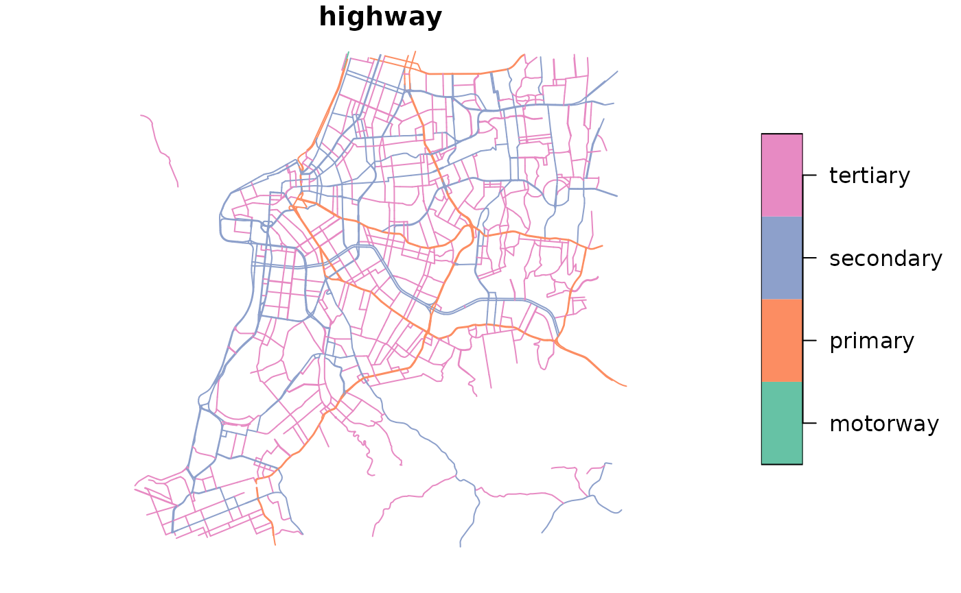
Then add a "max_speed" column by road type and a
speed_type column set to "scale", and make
osm_id numeric:
new_edge_speeds <- roads |>
  mutate(
    osm_id = as.numeric(osm_id),
    max_speed = case_when(
      highway == "motorway"  ~ 0.75,
      highway == "primary"   ~ 0.8,
      highway == "secondary" ~ 0.85,
      highway == "tertiary"  ~ 0.9)) |>
  sf::st_drop_geometry()

new_edge_speeds$speed_type <- "scale"

head(new_edge_speeds)
#>     osm_id highway max_speed speed_type
#> 1 26786712 primary       0.8      scale
#> 2 26786730 primary       0.8      scale
#> 3 26786732 primary       0.8      scale
#> 4 26847798 primary       0.8      scale
#> 5 26936215 primary       0.8      scale
#> 6 26936224 primary       0.8      scale
Travel times with the modified car speeds:
# travel time matrix
ttm_congestion <- r5r::travel_time_matrix(
  r5r_network = r5r_network,
  origins = points,
  destinations = points,
  mode = 'car',
  departure_datetime = Sys.time(),
  max_trip_duration = 30,
  new_carspeeds = new_edge_speeds
  )
2.1.2 Setting the same speed limit for the selected road types
To set a 40 km/h speed limit on the same road types (motorway,
primary, secondary, tertiary), set max_speed = 40 and
speed_type = "km/h" in the previous table:
# edit table with custom speeds to 40 km/h
new_edge_speeds40 <- new_edge_speeds |>
  mutate(max_speed = 40,
         speed_type = "km/h")

# travel time matrix
ttm_congestion <- r5r::travel_time_matrix(
  r5r_network = r5r_network,
  origins = points,
  destinations = points,
  mode = 'car',
  departure_datetime = Sys.time(),
  max_trip_duration = 30,
  new_carspeeds = new_edge_speeds40
  )
#> Warning: A scenario was used for this calculation. This may affect results for WALK or
#> BICYCLE due to missing elevation. See issue #555.2.2 Changing car speeds with a spatial polygon
Instead of listing OSM edges, you can set the speed of all roads within one or more polygons. The sample data has two polygons: one covering the extended city center, and one covering a few roads that connect two major avenues.
# read sf with congestion polygons
congestion_poly <- readRDS(file.path(data_path, "poa_poly_congestion.rds"))

# preview
mapview::mapview(congestion_poly, zcol="scale")
The sf data.frame must have these columns:
-
"poly_id": a unique id for each polygon -
"scale": the speed scaling factor for each polygon, relative to original speeds. Absolute speeds in km/h are not supported. -
"priority": a number ranking which polygon should be considered in case of overlapping polygons.
head(congestion_poly)
#> Simple feature collection with 2 features and 3 fields
#> Geometry type: POLYGON
#> Dimension:     XY
#> Bounding box:  xmin: -51.24537 ymin: -30.04352 xmax: -51.21426 ymax: -30.02548
#> Geodetic CRS:  WGS 84
#>   poly_id scale priority                       geometry
#> 1       1   0.7        1 POLYGON ((-51.22463 -30.034...
#> 2       2   0.8        2 POLYGON ((-51.21426 -30.034...
Here, roads in the city center run at 70% of the speed limit, roads
in the second polygon at 80%, and, with
carspeed_scale = 0.95, all other roads at 95%:
ttm_congestion <- r5r::travel_time_matrix(
  r5r_network = r5r_network,
  origins = points,
  destinations = points,
  mode = 'car',
  departure_datetime = Sys.time(),
  max_trip_duration = 30,
  new_carspeeds = congestion_poly,
  carspeed_scale = 0.95
  )
#> Warning: A scenario was used for this calculation. This may affect results for WALK or
#> BICYCLE due to missing elevation. See issue #555.
3. Changing cycling LTS values
LTS is changed like car speeds: with a data.frame of new
LTS values per OSM edge id, or with an sf data.frame. Here
the sf must be of type LINESTRING; R5 finds the nearest
road to each line and updates its LTS.
3.1 Changing LTS by OSM edge
Suppose protected cycle lanes or tracks were built on a few roads.
The data.frame must contain an "lts" column
with the new LTS value.
# read data.frame with new lts
edge_lts <- read.csv(
  file.path(data_path, "poa_osm_lts.csv")
  )

head(edge_lts)
#>      osm_id lts
#> 1  27184648   1
#> 2 762361901   1
#> 3 568609955   1
#> 4 709834913   1
#> 5 709834914   1
#> 6  77705540   1
Pass it to new_lts in any routing/accessibility
function:
ttm_new_lts <- r5r::travel_time_matrix(
  r5r_network = r5r_network,
  origins = points,
  destinations = points,
  mode = 'bicycle',
  departure_datetime = Sys.time(),
  max_trip_duration = 30,
  new_lts = edge_lts
  )
#> Warning: A scenario was used for this calculation. This may affect results for WALK or
#> BICYCLE due to missing elevation. See issue #555.
3.2. Changing LTS with spatial lines
Alternatively, pass an sf LINESTRING of the roads with
the intervention. Here, dedicated cycle lanes along all secondary
roads:
# read sf with congestion polygons
lts_lines <- readRDS(file.path(data_path, "poa_ls_lts.rds"))

# preview
mapview::mapview(lts_lines, zcol="lts")
Pass it to new_lts as before:
ttm_new_lts <- r5r::travel_time_matrix(
  r5r_network = r5r_network,
  origins = points,
  destinations = points,
  mode = 'bicycle',
  departure_datetime = Sys.time(),
  max_trip_duration = 30,
  new_lts = lts_lines
  )
#> Warning: A scenario was used for this calculation. This may affect results for WALK or
#> BICYCLE due to missing elevation. See issue #555.
Cleaning up after usage
Stop the network and run Java’s garbage collector to free the memory it used:
# stop an specific r5r network
r5r::stop_r5(r5r_network)

# or stop all r5r networks at once
r5r::stop_r5()
rJava::.jgc(R.gc = TRUE)
If you have any suggestions or want to report an error, please visit the package GitHub page.