Intro to r5r: Rapid Realistic Routing with R5 in R

Abstract

r5r is an R package for rapid realistic routing on multimodal transport networks (walk, bike, public transport and car) using R⁵. The package allows users to generate detailed routing analysis or calculate travel time matrices using seamless parallel computing on top of the R⁵ Java machine https://github.com/conveyal/r5

1. Introduction

r5r is an R package for rapid realistic routing on multimodal transport networks (walk, bike, public transport and car). It provides a simple and friendly interface to R⁵, a really fast and open source Java-based routing engine developed separately by Conveyal. R⁵ stands for Rapid Realistic Routing on Real-world and Reimagined networks. More details about r5r can be found on the package webpage or on this paper.

2. Installation

You can install r5r from CRAN, or the development version from github.

# from CRAN
install.packages('r5r')

# dev version with latest features
devtools::install_github("ipeaGIT/r5r", subdir = "r-package")

r5r requires the Java Development Kit (JDK) 21. Any free, open-source JDK works, for example:

Adoptium/Eclipse Temurin (our preferred option)
Amazon Corretto
Oracle OpenJDK.

The easiest way to install JDK 21 is with the {rJavaEnv} package in R:

# install {rJavaEnv} from CRAN
install.packages("rJavaEnv")

# check version of Java currently installed (if any) 
rJavaEnv::java_check_version_rjava()

## if this is the first time you use {rJavaEnv}, you might need to run this code
## below to consent the installation of Java.
# rJavaEnv::rje_consent(provided = TRUE)

# install Java 21
rJavaEnv::java_quick_install(version = 21)

# check if Java was successfully installed
rJavaEnv::java_check_version_rjava()

3. Usage

First, set the memory available to Java with the java.parameters option (2 GB is enough for the sample data). Do this before loading r5r or any other Java-based package: rJava starts the Java Virtual Machine only once per R session, so later changes only take effect after restarting R.

options(java.parameters = "-Xmx2G")

# By default, {r5r} uses all CPU cores available. If you want to limit the 
# number of CPUs to 4, for example, you can run:  
options(java.parameters = c("-Xmx2G", "-XX:ActiveProcessorCount=4"))

Then we can load the packages used in this vignette:

library(r5r)
library(sf)
library(data.table)
library(ggplot2)

r5r has eight fundamental functions:

Function	Returns
`build_network()`	A routable multimodal transport network
`accessibility()`	Access to opportunities from each origin, given a decay function
`travel_time_matrix()`	Travel times between origin/destination pairs for a departure time
`arrival_travel_time_matrix()`	Travel times for an arrival time, with routes used (and a time breakdown with `breakdown = TRUE`)
`expanded_travel_time_matrix()`	Travel times per departure minute, with routes used (and a time breakdown with `breakdown = TRUE`)
`detailed_itineraries()`	One or more alternative routes per origin/destination pair, detailed by trip segment
`pareto_frontier()`	The trade-off between travel time and monetary cost of route alternatives
`isochrone()`	Areas reachable from an origin within given travel times

Most of them can also account for monetary travel costs (fare structure vignette).

Support functions:

Function	Returns
`street_network_to_sf()`	The OpenStreetMap street network of a `network.dat` file, as `sf`
`transit_network_to_sf()`	The public transport network of a `network.dat` file, as `sf`
`find_snap()`	Where input points snap to the street network
`r5r_sitrep()`	A situation report to help debug errors

3.1 Data requirements:

To use r5r, you will need:

A road network data set from OpenStreetMap in .pbf format (mandatory)
A public transport feed in GTFS.zip format (optional)
A raster file of Digital Elevation Model data in .tif format (optional)

Here are a few places from where you can download these data sets:

OpenStreetMap
- osmextract R package
- geofabrik website
- hot export tool website
- BBBike.org website
GTFS
- tidytransit R package
- transitland website
- Mobility Database website
Elevation
- elevatr R package
- Nasa’s SRTMGL1 website

4. Demonstration on sample data

Data

r5r includes sample data for Porto Alegre (Brazil):

An OpenStreetMap network: poa_osm.pbf
Two public transport feeds: poa_eptc.zip and poa_trensurb.zip
A raster elevation data: poa_elevation.tif
A poa_hexgrid.csv file with spatial coordinates of a regular hexagonal grid covering the sample area, which can be used as origin/destination pairs in a travel time matrix calculation.
A poa_points_of_interest.csv file containing the names and spatial coordinates of 15 places within Porto Alegre
A fares_poa.zip file with the fare rules of the city’s public transport system.

data_path <- system.file("extdata/poa", package = "r5r")
list.files(data_path)
#>  [1] "fares"                      "gtfs_errors.csv"           
#>  [3] "network_settings.json"      "network.dat"               
#>  [5] "poa_elevation.tif"          "poa_eptc.zip"              
#>  [7] "poa_hexgrid.csv"            "poa_ls_lts.rds"            
#>  [9] "poa_osm_congestion.csv"     "poa_osm_lts.csv"           
#> [11] "poa_osm.pbf"                "poa_osm.pbf.mapdb"         
#> [13] "poa_osm.pbf.mapdb.p"        "poa_points_of_interest.csv"
#> [15] "poa_poly_congestion.rds"    "poa_trensurb.zip"          
#> [17] "r5r-log.log"

Points of interest, used below as origins and destinations:

poi <- fread(file.path(data_path, "poa_points_of_interest.csv"))
head(poi)
#>                     id       lat       lon
#>                 <char>     <num>     <num>
#> 1:       public_market -30.02756 -51.22781
#> 2: bus_central_station -30.02329 -51.21886
#> 3:    gasometer_museum -30.03404 -51.24095
#> 4: santa_casa_hospital -30.03043 -51.22240
#> 5:            townhall -30.02800 -51.22865
#> 6:     piratini_palace -30.03363 -51.23068

Hexagonal grid points; we use a random sample of 200:

points <- fread(file.path(data_path, "poa_hexgrid.csv"))

# sample points
sampled_rows <- sample(1:nrow(points), 200, replace = FALSE)
points <- points[ sampled_rows, ]
head(points)
#>                 id       lon       lat population schools  jobs healthcare
#>             <char>     <num>     <num>      <int>   <int> <int>      <int>
#> 1: 89a90128427ffff -51.20502 -30.08176        709       0     7          0
#> 2: 89a9012980fffff -51.17212 -30.02075       2073       0   127          0
#> 3: 89a90128043ffff -51.18627 -30.06949         21       1   100          0
#> 4: 89a9012828fffff -51.17700 -30.06612        965       0   219          0
#> 5: 89a90128657ffff -51.16852 -30.08209        678       0     0          0
#> 6: 89a9012826bffff -51.16740 -30.05445        240       1   180          0

4.1 Building routable transport network with `build_network()`

build_network() (1) downloads the R⁵ JAR (on first use or when the R⁵ version changes) and caches it locally; and (2) combines the .pbf, GTFS .zip and optional elevation .tif files in data_path into a routable network.

# Indicate the path where OSM and GTFS data are stored
r5r_network <- build_network(data_path = data_path)

4.2 Accessibility analysis

accessibility() is the fastest way to estimate accessibility. Here we count the schools and healthcare facilities reachable in less than 60 minutes by public transport and walking (accessibility vignette).

# set departure datetime input
departure_datetime <- as.POSIXct("13-05-2019 14:00:00",
                                 format = "%d-%m-%Y %H:%M:%S")

# calculate accessibility
access <- accessibility(
  r5r_network,
  origins = points,
  destinations = points,
  opportunities_colnames = c("schools", "healthcare"),
  mode = c("WALK", "TRANSIT"),
  departure_datetime = departure_datetime,
  decay_function = "step",
  cutoffs = 60
  )

head(access)
#>                 id opportunity percentile cutoff accessibility
#>             <char>      <char>      <int>  <int>         <num>
#> 1: 89a90128427ffff     schools         50     60            27
#> 2: 89a90128427ffff  healthcare         50     60            27
#> 3: 89a9012980fffff     schools         50     60            22
#> 4: 89a9012980fffff  healthcare         50     60            23
#> 5: 89a90128043ffff     schools         50     60            31
#> 6: 89a90128043ffff  healthcare         50     60            29

4.3 Routing analysis

For fast routing analysis, r5r currently has three core functions: travel_time_matrix(), expanded_travel_time_matrix() and detailed_itineraries().

Fast many to many travel time matrix

travel_time_matrix() computes travel times between origin/destination pairs. Origins and destinations can be an sf POINT object or a data.frame with columns id, lon and lat. max_walk_time and max_trip_duration are in minutes, as are the resulting travel times.

It can also capture travel time variation across departures within a time window (time window vignette).

# set inputs
mode <- c("WALK", "TRANSIT")
max_walk_time <- 30 # minutes
max_trip_duration <- 120 # minutes
departure_datetime <- as.POSIXct("13-05-2019 14:00:00",
                                 format = "%d-%m-%Y %H:%M:%S")

# calculate a travel time matrix
ttm <- travel_time_matrix(
  r5r_network,
  origins = poi,
  destinations = poi,
  mode = mode,
  departure_datetime = departure_datetime,
  max_walk_time = max_walk_time,
  max_trip_duration = max_trip_duration
  )

head(ttm)
#>          from_id               to_id travel_time_p50
#>           <char>              <char>           <int>
#> 1: public_market       public_market               0
#> 2: public_market bus_central_station              14
#> 3: public_market    gasometer_museum              12
#> 4: public_market santa_casa_hospital              15
#> 5: public_market            townhall               3
#> 6: public_market     piratini_palace              17

Expanded travel time matrix with minute-by-minute estimates

expanded_travel_time_matrix() works like travel_time_matrix() but also returns, for each origin/destination pair, the routes used and (with breakdown = TRUE) the access, waiting, in-vehicle and transfer times. It can be very memory intensive for large data sets.

# calculate a travel time matrix
ettm <- expanded_travel_time_matrix(
  r5r_network,
  origins = poi,
  destinations = poi,
  mode = mode,
  departure_datetime = departure_datetime,
  breakdown = TRUE,
  max_walk_time = max_walk_time,
  max_trip_duration = max_trip_duration
  )

head(ettm)
#>          from_id         to_id departure_time draw_number access_time wait_time
#>           <char>        <char>         <char>       <int>       <num>     <num>
#> 1: public_market public_market       14:00:00           1           0         0
#> 2: public_market public_market       14:01:00           1           0         0
#> 3: public_market public_market       14:02:00           1           0         0
#> 4: public_market public_market       14:03:00           1           0         0
#> 5: public_market public_market       14:04:00           1           0         0
#> 6: public_market public_market       14:05:00           1           0         0
#>    ride_time transfer_time egress_time routes n_rides total_time
#>        <num>         <num>       <num> <char>   <int>      <num>
#> 1:         0             0           0 [WALK]       0          0
#> 2:         0             0           0 [WALK]       0          0
#> 3:         0             0           0 [WALK]       0          0
#> 4:         0             0           0 [WALK]       0          0
#> 5:         0             0           0 [WALK]       0          0
#> 6:         0             0           0 [WALK]       0          0

Detailed itineraries

Most routing packages return only the fastest route. detailed_itineraries() can also return alternative routes between origin/destination pairs, detailed by trip segment: transport mode, waiting time, travel time and distance.

Below, alternative routes for a single origin/destination pair:

# set inputs
origins <- poi[10,]
destinations <- poi[12,]
mode <- c("WALK", "TRANSIT")
max_walk_time <- 60 # minutes
departure_datetime <- as.POSIXct("13-05-2019 14:00:00",
                                 format = "%d-%m-%Y %H:%M:%S")

# calculate detailed itineraries
det <- detailed_itineraries(
  r5r_network,
  origins = origins,
  destinations = destinations,
  mode = mode,
  departure_datetime = departure_datetime,
  max_walk_time = max_walk_time,
  shortest_path = FALSE
  )

head(det)
#> Simple feature collection with 6 features and 16 fields
#> Geometry type: LINESTRING
#> Dimension:     XY
#> Bounding box:  xmin: -51.24094 ymin: -30.05 xmax: -51.19762 ymax: -29.99729
#> Geodetic CRS:  WGS 84
#>            from_id  from_lat  from_lon                          to_id    to_lat
#> 1 farrapos_station -29.99772 -51.19762 praia_de_belas_shopping_center -30.04995
#> 2 farrapos_station -29.99772 -51.19762 praia_de_belas_shopping_center -30.04995
#> 3 farrapos_station -29.99772 -51.19762 praia_de_belas_shopping_center -30.04995
#> 4 farrapos_station -29.99772 -51.19762 praia_de_belas_shopping_center -30.04995
#> 5 farrapos_station -29.99772 -51.19762 praia_de_belas_shopping_center -30.04995
#> 6 farrapos_station -29.99772 -51.19762 praia_de_belas_shopping_center -30.04995
#>      to_lon option departure_time total_duration total_distance segment mode
#> 1 -51.22875      1       14:07:57           35.6           9460       1 WALK
#> 2 -51.22875      1       14:07:57           35.6           9460       2 RAIL
#> 3 -51.22875      1       14:07:57           35.6           9460       3 WALK
#> 4 -51.22875      1       14:07:57           35.6           9460       4  BUS
#> 5 -51.22875      1       14:07:57           35.6           9460       5 WALK
#> 6 -51.22875      2       14:09:43           46.0           8779       1 WALK
#>   segment_duration wait distance  route                       geometry
#> 1              5.1  0.0      174        LINESTRING (-51.1981 -29.99...
#> 2              6.6  2.0     4796 LINHA1 LINESTRING (-51.19763 -29.9...
#> 3              4.0  0.0      256        LINESTRING (-51.22827 -30.0...
#> 4             10.4  4.4     4083    188 LINESTRING (-51.22926 -30.0...
#> 5              3.2  0.0      151        LINESTRING (-51.22949 -30.0...
#> 6              5.1  0.0      174        LINESTRING (-51.1981 -29.99...

The output is an sf data.frame, ready to map.

Visualize results

street_network_to_sf() extracts the OSM street network used in routing, to give the map geographic context:

# extract OSM network
street_net <- r5r::street_network_to_sf(r5r_network)

# extract public transport network
transit_net <- r5r::transit_network_to_sf(r5r_network)

# plot
ggplot() +
  geom_sf(data = street_net$edges, color='gray85') +
  geom_sf(data = det, aes(color=mode)) +
  facet_wrap(.~option) + 
  theme_void()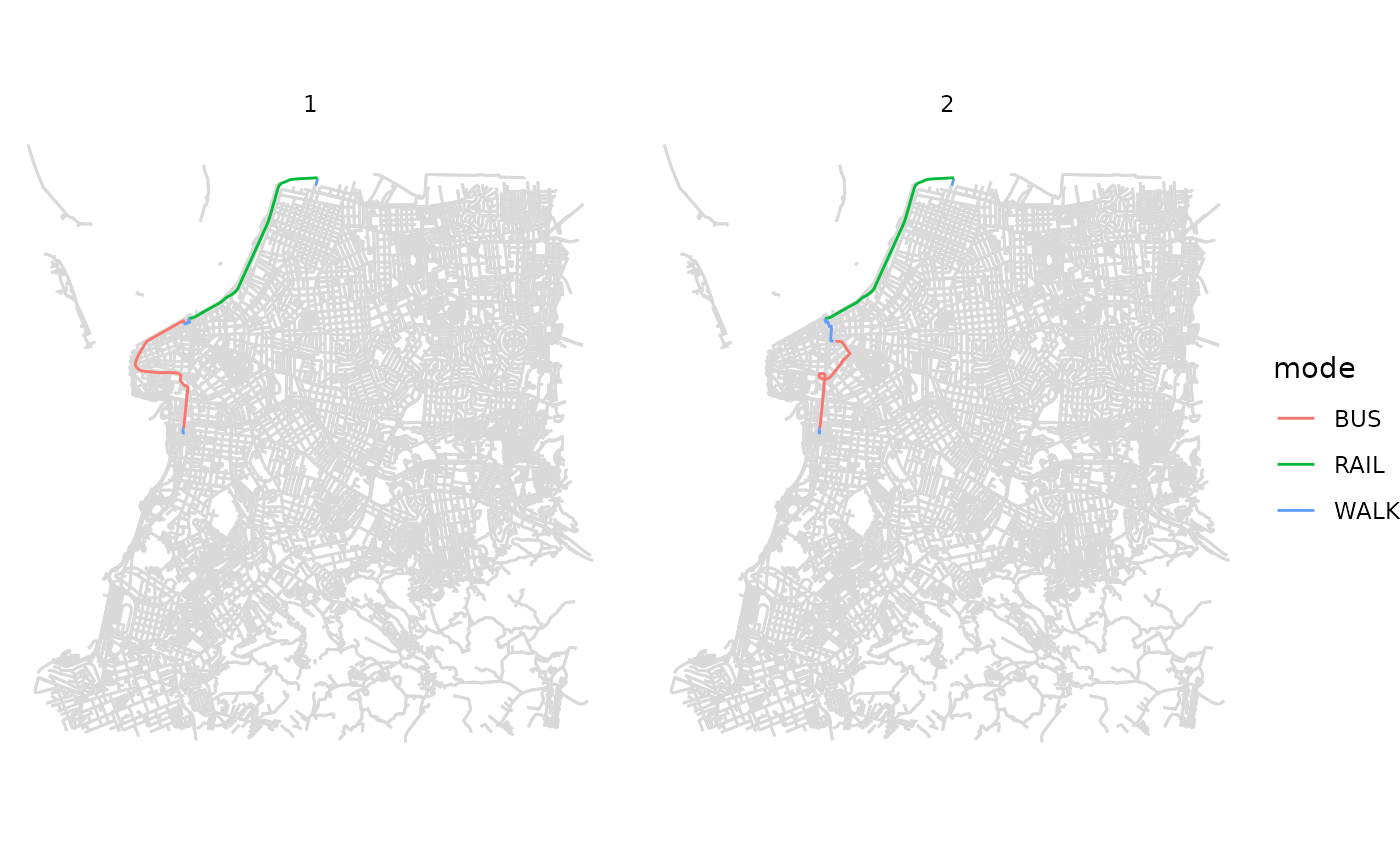

Cleaning up after usage

Stop the network and run Java’s garbage collector to free the memory it used:

r5r::stop_r5(r5r_network)
rJava::.jgc(R.gc = TRUE)

If you have any suggestions or want to report an error, please visit the package GitHub page.

Rafael H. M. Pereira, Marcus Saraiva, Daniel Herszenhut, Carlos Kaue Braga

2026-10-10

1. Introduction

2. Installation

3. Usage

3.1 Data requirements:

4. Demonstration on sample data

Data

4.1 Building routable transport network with `build_network()`

4.2 Accessibility analysis

4.3 Routing analysis

Fast many to many travel time matrix

Expanded travel time matrix with minute-by-minute estimates

Detailed itineraries

Visualize results

Cleaning up after usage

Intro to r5r: Rapid Realistic Routing with R5 in R

Rafael H. M. Pereira, Marcus Saraiva, Daniel Herszenhut, Carlos Kaue Braga

2026-10-10

1. Introduction

2. Installation

3. Usage

3.1 Data requirements:

4. Demonstration on sample data

Data

4.1 Building routable transport network with build_network()

4.2 Accessibility analysis

4.3 Routing analysis

Fast many to many travel time matrix

Expanded travel time matrix with minute-by-minute estimates

Detailed itineraries

Visualize results

Cleaning up after usage

4.1 Building routable transport network with `build_network()`