
Abstract
This vignette shows how to calculate and visualize isochrones in R using ther5r package.
1. Introduction
An isochrone shows all areas reachable from a place within a maximum
travel time. This vignette uses the r5r
package and the Porto Alegre (Brazil) sample data included in it to
calculate and map public transport isochrones from the city’s central
bus station at several travel time thresholds.
r5r::isochrone() builds both polygon- and line-based
isochrones; we cover both.
Warning: to count opportunities (e.g. jobs,
schools or hospitals) within each isochrone, we strongly recommend NOT
using isochrone(). The Accessibility
vignette shows much more efficient ways.
2. Build routable transport network with
build_network()
Increase Java memory and load libraries
Set Java memory before loading the packages (why).
build_network() takes the directory holding the
OpenStreetMap and GTFS data:
# system.file returns the directory with example data inside the r5r package
# set data path to directory containing your own data if not running this example
data_path <- system.file("extdata/poa", package = "r5r")

r5r_network <- build_network(data_path)
3. Calculating and visualizing isochrones
3.1 Polygon-based isochrones
Polygon-based isochrones are the most common: set
polygon_output = TRUE. The polygons are built on a regular
grid of Web
Mercator pixels whose resolution is set by zoom. Higher
zooms give more detailed isochrones but take longer, and may fail with
an error in large networks. The default, 10, uses cells of 153 m at the
Equator.
Below, isochrones use the median travel time of departures every minute over a 60-minute window (2pm to 3pm).
# read all points in the city
points <- fread(file.path(data_path, "poa_hexgrid.csv"))

# subset point with the geolocation of the central bus station
central_bus_stn <- points[291,]

# isochrone intervals
time_intervals <- seq(0, 100, 10)

# routing inputs
mode <- c("WALK", "TRANSIT")
max_walk_time <- 30      # in minutes
time_window <- 60        # in minutes
departure_datetime <- as.POSIXct("13-05-2019 14:00:00",
                                 format = "%d-%m-%Y %H:%M:%S")

# calculate travel time matrix
iso1 <- r5r::isochrone(
  r5r_network,
  origins = central_bus_stn,
  mode = mode,
  polygon_output = TRUE,
  cutoffs = time_intervals,
  departure_datetime = departure_datetime,
  max_walk_time = max_walk_time,
  time_window = time_window,
  progress = FALSE,
  zoom = 10
  )
isochrone() works like
travel_time_matrix(), but with
polygon_output = TRUE it returns an sf
data.frame with one POLYGON/MULTIPOLYGON per
origin, cutoff and percentile:
head(iso1)
#> Simple feature collection with 6 features and 3 fields
#> Geometry type: MULTIPOLYGON
#> Dimension:     XY
#> Bounding box:  xmin: -51.26701 ymin: -30.11365 xmax: -51.13243 ymax: -29.99003
#> Geodetic CRS:  WGS 84
#>                id isochrone percentile                       polygons
#> 1 89a90128a8fffff       100        p50 MULTIPOLYGON (((-51.14891 -...
#> 2 89a90128a8fffff        90        p50 MULTIPOLYGON (((-51.16493 -...
#> 3 89a90128a8fffff        80        p50 MULTIPOLYGON (((-51.16814 -...
#> 4 89a90128a8fffff        70        p50 MULTIPOLYGON (((-51.17638 -...
#> 5 89a90128a8fffff        60        p50 MULTIPOLYGON (((-51.22444 -...
#> 6 89a90128a8fffff        50        p50 MULTIPOLYGON (((-51.22581 -...
Mapping the isochrones:
# extract OSM network
street_net <- street_network_to_sf(r5r_network)
main_roads <- subset(street_net$edges, street_class %like% 'PRIMARY|SECONDARY')
colors <- c('#ffe0a5','#ffcb69','#ffa600','#ff7c43','#f95d6a',
'#d45087','#a05195','#665191','#2f4b7c','#003f5c')
ggplot() +
geom_sf(data = iso1, aes(fill=factor(isochrone)), color = NA, alpha = .7) +
geom_sf(data = main_roads, color = "gray55", size=0.01, alpha = 0.2) +
geom_point(data = central_bus_stn, aes(x=lon, y=lat, color='Central bus\nstation')) +
scale_fill_manual(values = rev(colors) ) +
scale_color_manual(values=c('Central bus\nstation'='black')) +
labs(fill = "Travel time\n(in minutes)", color='') +
theme_minimal() +
theme(axis.title = element_blank())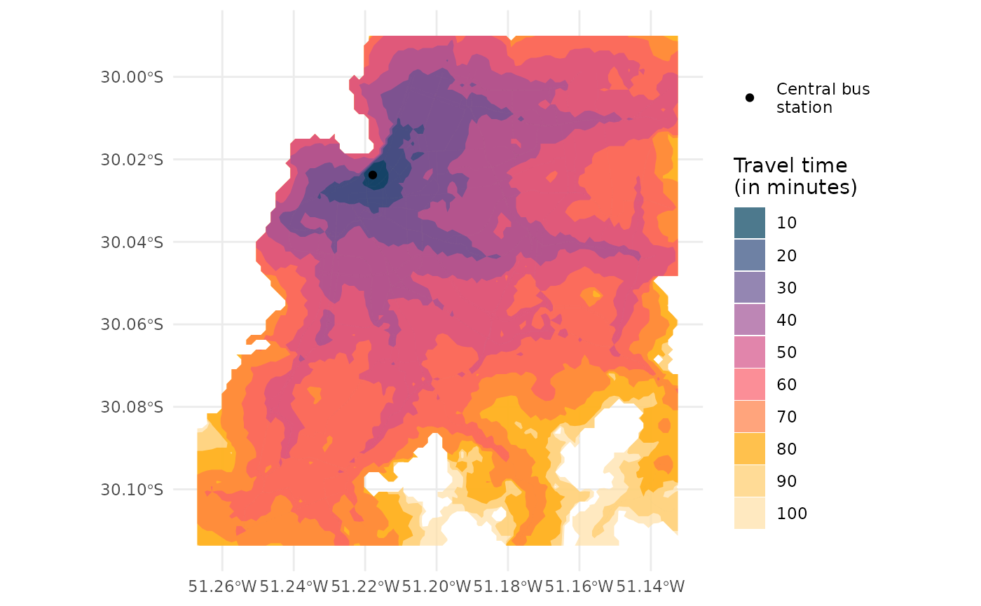 ## 3.2 Line-based isochrones
For line-based isochrones, set polygon_output = FALSE
(no zoom needed). The output is a LINESTRING
sf data.frame.
# calculate travel time matrix
iso2 <- r5r::isochrone(
  r5r_network,
  origins = central_bus_stn,
  mode = mode,
  polygon_output = FALSE,
  cutoffs = time_intervals,
  departure_datetime = departure_datetime,
  max_walk_time = max_walk_time,
  time_window = time_window,
  progress = FALSE
  )

head(iso2)
#> Simple feature collection with 6 features and 14 fields
#> Geometry type: LINESTRING
#> Dimension:     XY
#> Bounding box:  xmin: -51.20291 ymin: -30.10872 xmax: -51.1844 ymax: -30.09557
#> Geodetic CRS:  WGS 84
#>                id edge_index    osm_id isochrone travel_time_p50 from_vertex
#> 1 89a90128a8fffff      32820 289389686       100              98        7464
#> 2 89a90128a8fffff      32821 289389686       100              98       14753
#> 3 89a90128a8fffff      34254 326021940       100              98       15308
#> 4 89a90128a8fffff      34255 326021940       100              98       15309
#> 5 89a90128a8fffff      35888 337865739       100              98       15671
#> 6 89a90128a8fffff      35889 337865739       100              98       15690
#>   to_vertex street_class  length  walk   car car_speed bicycle bicycle_lts
#> 1     14753        OTHER 374.345  TRUE  TRUE    39.996    TRUE           2
#> 2      7464        OTHER 374.345  TRUE  TRUE    39.996    TRUE           2
#> 3     15309        OTHER 227.438  TRUE FALSE    40.248    TRUE           1
#> 4     15308        OTHER 227.438  TRUE FALSE    40.248    TRUE           1
#> 5     15690        OTHER  87.668 FALSE FALSE    40.248   FALSE           1
#> 6     15671        OTHER  87.668 FALSE FALSE    40.248   FALSE           1
#>                         geometry
#> 1 LINESTRING (-51.19973 -30.1...
#> 2 LINESTRING (-51.20291 -30.1...
#> 3 LINESTRING (-51.1844 -30.10...
#> 4 LINESTRING (-51.18581 -30.1...
#> 5 LINESTRING (-51.19704 -30.0...
#> 6 LINESTRING (-51.19686 -30.0...
Mapping the isochrones:
ggplot() +
  geom_sf(data = iso2, aes(color=factor(isochrone)), alpha = .7) +
  scale_color_manual(values = rev(colors) ) +
  geom_point(data = central_bus_stn, aes(x=lon, y=lat), color='black') +
  labs(color = "Travel time\n(in minutes)") +
  theme_minimal() +
  theme(axis.title = element_blank())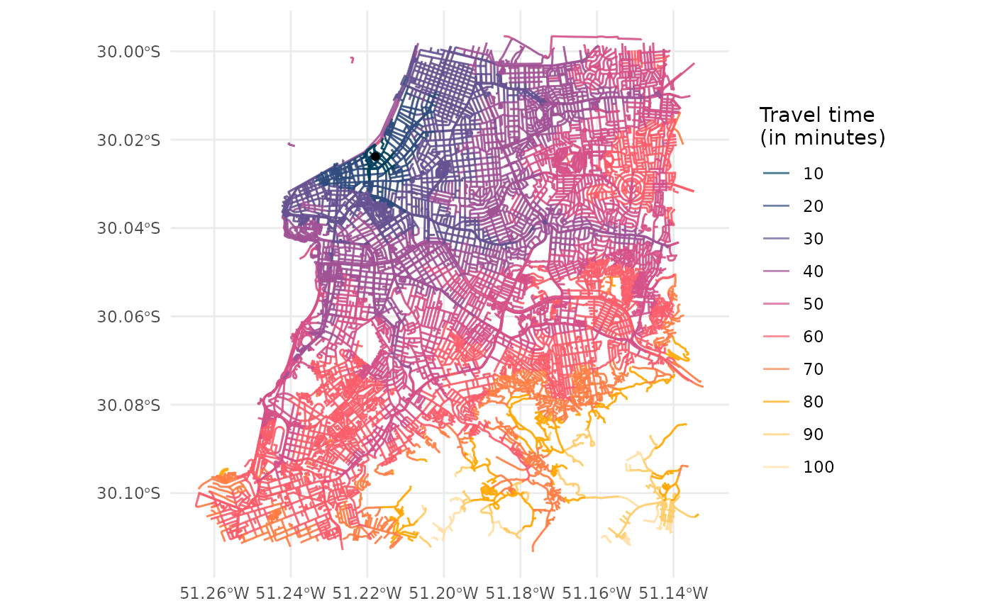
Cleaning up after usage
Stop the network and run Java’s garbage collector to free the memory it used:
If you have any suggestions or want to report an error, please visit the package GitHub page.