Accounting for monetary costs

Abstract

This vignette shows how to configure and use custom fare rules in order to account for monetary travel costs when generating travel time matrices and accessibility estimates with the r5r package.

1. Introduction

Accounting for the monetary cost of public transport trips in travel time matrices and accessibility estimates is a major challenge. Fare rules vary across systems and can be complex, and the trade-offs between travel time and cost across trip alternatives are not captured by any multimodal routing engine except R5.

R5 can combine time and monetary cost cutoffs, but each city’s fare structure must be programmed in Java and integrated into R5. Instead, r5r offers a generic rule-based fare structure that you configure from R, or with a text editor or spreadsheet. It covers systems where the cost of a journey depends on combinations of modes (see details below).

This vignette describes r5r’s fare structure and shows, with a reproducible example, how to configure it to account for monetary costs in travel time matrices and accessibility estimates.

1.1 Details

Supported: discounted transfers. A single ticket covers a trip of several rides, possibly on different modes, with a discount on the second or subsequent fares, optionally limited in the number of discounted transfers and/or in time. Fares can differ by mode, agency or route (see by and use_route_fare below).

Not supported: more complex rules, such as:

distance- or zone-based fares;
fares by type of rider (e.g. elderly people or students);
fares by time of day (e.g. peak and off-peak hours).

The fare calculator is not meant to cover every public transport system. Its features are based on systems that use discounted transfers, which is a widely common system across many cities; everyone is welcome to use it if it suits their needs.

obs. GTFS fare features are too limited for many use cases. A new specification, Fares V2, is being developed, but it may take time to be approved and adopted by transport agencies.

2. Reprex: the public transport system of Porto Alegre

In this vignette, we will be using the sample data set for the city of Porto Alegre (Brazil) included in r5r. Set Java memory before loading the packages (why).

options(java.parameters = "-Xmx2G")

library(r5r)
library(sf)
library(data.table)
library(ggplot2)
library(patchwork)
library(dplyr)
library(h3jsr)

Porto Alegre’s public transport is mostly buses, plus a metropolitan rail line connecting the city center to municipalities to the north:

# setup and load Porto Alegre multimodal network into memory

# system.file returns the directory with example data inside the r5r package
# set data path to directory containing your own data if not using the examples
data_path <- system.file("extdata/poa", package = "r5r")

r5r_network <- build_network(data_path)
#> Using cached R5 version from /home/runner/.cache/R/r5r/r5_jar_v7.5.1/r5-v7.5-1-gf3631e9-all.jar
#> ℹ Using cached network from
#>   /home/runner/work/_temp/Library/r5r/extdata/poa/network.dat.

# load transit network as an SF
transit_network <- transit_network_to_sf(r5r_network)

# map
ggplot() +
  geom_sf(data=transit_network$routes, aes(color=mode)) +
  theme_void()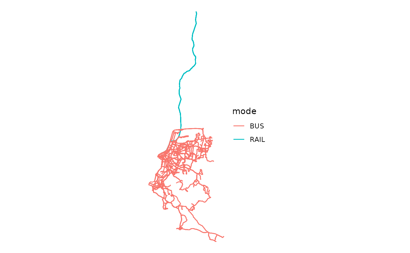

As in most Brazilian cities, the cost of a journey depends on the number of rides and the modes combined:

Each bus ticket costs R$ 4.80.
Riding a second bus adds R$ 2.40 to the total cost. Subsequent bus rides cost the full ticket price of R$ 4.80.
Each train ticket costs R$ 4.50. Once a passenger enters a train station, she can take an unlimited amount of train trips as long as she doesn’t leave a station.
The integrated fare between bus and train has a 10% discount, which totals R$ 8.37.

3. Setting up the fare structure

Three functions help configure the fare structure:

setup_fare_structure() analyses the study area’s GTFS and builds a ‘skeleton’ fare structure with the parameters to set;
write_fare_structure() and read_fare_structure() save the fare structure to disk and read it back. It is stored as .csv files in a .zip, which you can also edit in a text editor or spreadsheet.

setup_fare_structure() takes the r5r_network, a base_fare to populate the structure, and by, the route property that defines different fares. Below, base_fare is the bus ticket price (R$ 4.80) and by = "MODE" gives each mode its own fares and transfer rules. Fares can also differ by "AGENCY_ID" or "AGENCY_NAME"; use by = "GENERIC" if the whole system follows the same rules.

fare_structure <- setup_fare_structure(r5r_network,
                                       base_fare = 4.8,
                                       by = "MODE")

fare_structure is a list of global properties and data.frames:

head(fare_structure, n=7)
#> $max_discounted_transfers
#> [1] 1
#> 
#> $transfer_time_allowance
#> [1] 120
#> 
#> $fare_cap
#> [1] Inf
#> 
#> $fares_per_type
#>      type unlimited_transfers allow_same_route_transfer use_route_fare  fare
#>    <char>              <lgcl>                    <lgcl>         <lgcl> <num>
#> 1:    BUS               FALSE                     FALSE          FALSE   4.8
#> 2:   RAIL               FALSE                     FALSE          FALSE   4.8
#> 
#> $fares_per_transfer
#>    first_leg second_leg  fare
#>       <char>     <char> <num>
#> 1:       BUS        BUS   4.8
#> 2:      RAIL        BUS   4.8
#> 3:       BUS       RAIL   4.8
#> 4:      RAIL       RAIL   4.8
#> 
#> $fares_per_route
#>      agency_id                                 agency_name  route_id
#>         <char>                                      <char>    <char>
#>   1:     TRENS                                    TRENSURB    LINHA1
#>   2:     TRENS                                    TRENSURB LINHAAERO
#>   3:      EPTC Empresa Publica de Transportes e Circulação      1112
#>   4:      EPTC Empresa Publica de Transportes e Circulação       149
#>   5:      EPTC Empresa Publica de Transportes e Circulação       165
#>  ---                                                                
#> 113:      EPTC Empresa Publica de Transportes e Circulação        T7
#> 114:      EPTC Empresa Publica de Transportes e Circulação        T8
#> 115:      EPTC Empresa Publica de Transportes e Circulação        T9
#> 116:      EPTC Empresa Publica de Transportes e Circulação      TR60
#> 117:      EPTC Empresa Publica de Transportes e Circulação      TR62
#>      route_short_name                           route_long_name   mode
#>                <char>                                    <char> <char>
#>   1:           LINHA1 ESTACAO MERCADO ATE ESTACAO NOVO HAMBURGO   RAIL
#>   2:             AREO                        AEROMOVEL TRENSURB   RAIL
#>   3:             1112                         HIPICA / TRISTEZA    BUS
#>   4:              149                                    ICARAI    BUS
#>   5:              165                                     COHAB    BUS
#>  ---                                                                  
#> 113:               T7                     NILO / PRAIA DE BELAS    BUS
#> 114:               T8                       CAMPUS  /  FARRAPOS    BUS
#> 115:               T9                                       PUC    BUS
#> 116:             TR60                         TRONCAL TRI‘NGULO    BUS
#> 117:             TR62                          TRONCAL BALTAZAR    BUS
#>      route_fare fare_type
#>           <num>    <char>
#>   1:        4.8      RAIL
#>   2:        4.8      RAIL
#>   3:        4.8       BUS
#>   4:        4.8       BUS
#>   5:        4.8       BUS
#>  ---                     
#> 113:        4.8       BUS
#> 114:        4.8       BUS
#> 115:        4.8       BUS
#> 116:        4.8       BUS
#> 117:        4.8       BUS
#> 
#> $debug_settings
#> $debug_settings$output_file
#> [1] ""
#> 
#> $debug_settings$trip_info
#> [1] "MODE"

3.1 Global Properties

Global properties apply to the entire system.

`max_discounted_transfers`

Note that max_discounted_transfers is set to 1 by default. This means that the passenger gets a fare discount in the first transfer between buses, but she would pay the full fare price in subsequent transfers.

`transfer_time_allowance`

By default, transfer_time_allowance is set to 120 minutes. We have to set it to 60 minutes to fit our use case (passengers have 60 minutes to take the second bus on a discounted fare, otherwise a full fare is charged).

`fare_cap`

Finally, the fare_cap setting indicates if there is a maximum value that can be charged in a trip, beyond which all subsequent rides are free of charge. In this example, we can leave fare_cap set to its default Inf value because this feature is not applicable to Porto Alegre.

To check or update them:

fare_structure$max_discounted_transfers
#> [1] 1
fare_structure$transfer_time_allowance <- 60 # update transfer_time_allowance
fare_structure$fare_cap
#> [1] Inf

3.2 Configure fares by transport mode

To configure mode-, transfer-, and route-specific properties, we can use the three data.frames inside our fare_structure list. Let’s configure the modes first. Below, we can see that the fares_per_type data.frame contains five columns:

mode: the transport mode to which rules on each row refer to;
unlimited_transfers: a logical value TRUE or FALSE that indicates if that transport mode allows unlimited transfers between trips of the same mode, such as a metro/subway system where the passenger pays a fare to access a station and then can use as many services as she wants as long as she doesn’t exit the system;
allow_same_route_transfer: a logical value indicating if a discounted transfer can be done between vehicles of the same route;
use_route_fare: another logical value that indicates if each route will have its own fare, or if all routes in this mode will use the fare indicated in this table;
fare: the full fare price of this mode.

fare_structure$fares_per_type
#>      type unlimited_transfers allow_same_route_transfer use_route_fare  fare
#>    <char>              <lgcl>                    <lgcl>         <lgcl> <num>
#> 1:    BUS               FALSE                     FALSE          FALSE   4.8
#> 2:   RAIL               FALSE                     FALSE          FALSE   4.8

To accommodate the fare rules of Porto Alegre, we set unlimited_transfers and allow_same_route_transfer to TRUE and fare to 4.50 for "RAIL". For "BUS", keep the default allow_same_route_transfer = FALSE: the bus-to-bus discount (set in the next section) does not apply between buses of the same route (e.g. from route T1 to another T1). In data.table notation:

fare_structure$fares_per_type[type == "RAIL", unlimited_transfers := TRUE]
fare_structure$fares_per_type[type == "RAIL", fare := 4.50]
fare_structure$fares_per_type[type == "RAIL", allow_same_route_transfer := TRUE]

The result:

fare_structure$fares_per_type
#> Index: <type>
#>      type unlimited_transfers allow_same_route_transfer use_route_fare  fare
#>    <char>              <lgcl>                    <lgcl>         <lgcl> <num>
#> 1:    BUS               FALSE                     FALSE          FALSE   4.8
#> 2:   RAIL                TRUE                      TRUE          FALSE   4.5

3.3 Configure fares by transfers

The fare rules for transfer are stored in the fares_per_transfer data.frame, which is shown below. Each row contains the fare prices for transfers between the modes specified in first_leg and second_leg columns.

fare_structure$fares_per_transfer
#>    first_leg second_leg  fare
#>       <char>     <char> <num>
#> 1:       BUS        BUS   4.8
#> 2:      RAIL        BUS   4.8
#> 3:       BUS       RAIL   4.8
#> 4:      RAIL       RAIL   4.8

Let’s update fare_per_transfer to account for the actual integration rules in Porto Alegre.

The fare for “BUS” to “BUS” integration is composed of 4.80 for the first leg plus 2.40 for the second leg, which equals to a total fare of 7.20.

# conditional update fare value
fare_structure$fares_per_transfer[first_leg == "BUS" & second_leg == "BUS", fare := 7.2]

Transfers between “BUS” and “RAIL” (in any direction) cost 8.37, once the 10% discount is applied. Let’s make a final update in the data.frame to account for that.

# conditional update fare value
fare_structure$fares_per_transfer[first_leg != second_leg, fare := 8.37]

# use fcase instead ?
fare_structure$fares_per_transfer[, fare := fcase(first_leg == "BUS" & second_leg == "BUS", 7.2,
                                                 first_leg != second_leg, 8.37)]

Transfers between “RAIL” and “RAIL” are free and unlimited, which is already accounted for in the field unlimited_transfers of the fare_per_mode table. Thus, the equivalent row of the fare_per_transfer data.frame needs to be removed. If we leave the that row in fare_per_transfer, transfers between “RAIL” and “RAIL” will count to the global max_discounted_transfers allowance.

# remove row
fare_structure$fares_per_transfer <- fare_structure$fares_per_transfer[!(first_leg == "RAIL" & second_leg == "RAIL")]

Once all changes are applied, the fare_per_transfer data.frame should look like this:

fare_structure$fares_per_transfer
#>    first_leg second_leg  fare
#>       <char>     <char> <num>
#> 1:       BUS        BUS  7.20
#> 2:      RAIL        BUS  8.37
#> 3:       BUS       RAIL  8.37

3.4 Routes configuration

The information on the fare price for each route is stored in the fares_per_route data.frame. Below, we can see a sample of the bus and train routes in Porto Alegre. In case there a few special routes (e.g. express services) with specific fares, these values can be updated in this fares_per_route data.frame.

tail(fare_structure$fares_per_route)
#>    agency_id                                 agency_name route_id
#>       <char>                                      <char>   <char>
#> 1:      EPTC Empresa Publica de Transportes e Circulação       T6
#> 2:      EPTC Empresa Publica de Transportes e Circulação       T7
#> 3:      EPTC Empresa Publica de Transportes e Circulação       T8
#> 4:      EPTC Empresa Publica de Transportes e Circulação       T9
#> 5:      EPTC Empresa Publica de Transportes e Circulação     TR60
#> 6:      EPTC Empresa Publica de Transportes e Circulação     TR62
#>    route_short_name       route_long_name   mode route_fare fare_type
#>              <char>                <char> <char>      <num>    <char>
#> 1:               T6         TRANSVERSAL 6    BUS        4.8       BUS
#> 2:               T7 NILO / PRAIA DE BELAS    BUS        4.8       BUS
#> 3:               T8   CAMPUS  /  FARRAPOS    BUS        4.8       BUS
#> 4:               T9                   PUC    BUS        4.8       BUS
#> 5:             TR60     TRONCAL TRI‘NGULO    BUS        4.8       BUS
#> 6:             TR62      TRONCAL BALTAZAR    BUS        4.8       BUS

Basic route information is taken directly from the GTFS data (agency, route id and names, mode, etc), but the route_fare and fare_type columns were added specifically for the r5r fare structure.

route_fare: is used to set a specific fare for each route. This field can be used to represent services that have many unique fares, such as metropolitan / suburban trains and buses. This is used together with the use_route_fare column in the fares_per_type table: the route_fare field is only considered by the r5r fare structure when use_route_fare of that mode is set to TRUE.
fare_type: is used to link each route with information in the fares_per_type and fares_per_transfer tables. In this example, fare_type is always the same as mode, because that was what we chose in the by parameter when calling setup_fare_structure earlier (we could have chosen to discriminate fares by agency, for example).

No changes to fares_per_route are needed here. The route_fare values of the “RAIL” lines are wrong, but they are not used because use_route_fare is FALSE for RAIL: fares come from fares_per_type and fares_per_transfer, set above. The fare_structure is now complete.

4. Calculating travel time and accessibility accounting for monetary costs

travel_time_matrix() and accessibility() take two parameters for monetary cost thresholds:

fare_structure: the settings object that we’ve been working on.
max_fare: the maximum total fare that can be used in the trip.

4.1 Travel time with monetary cost

Travel times with and without a R$ 5.00 fare limit:

## load input data
points <- read.csv(system.file("extdata/poa/poa_hexgrid.csv", package = "r5r"))

# calculate travel times function
calculate_travel_times <- function(fare) {
  ttm_df <- travel_time_matrix(
    r5r_network,
    origins = points,
    destinations = points,
    mode = c("WALK", "TRANSIT"),
    departure_datetime = as.POSIXct(
      "13-05-2019 14:00:00",
      format = "%d-%m-%Y %H:%M:%S"
    ),
    time_window = 1,
    fare_structure = fare_structure,
    max_fare = fare,
    max_trip_duration = 40,
    max_walk_time = 20
  )

  return(ttm_df)
}


# calculate travel times, and combine results
ttm <- calculate_travel_times(fare = Inf)
#> Loading required namespace: testthat
ttm_500 <- calculate_travel_times(fare = 5)

# merge results
ttm[ttm_500, on = .(from_id, to_id), travel_time_500 := i.travel_time_p50]
ttm[, travel_time_unl := travel_time_p50]
ttm[, travel_time_p50 := NULL]

Some trips are unaffected (travel_time_unl == travel_time_500), some take longer (travel_time_500 > travel_time_unl), and some cannot be completed (travel_time_500 == NA):

tail(ttm, 10)
#>             from_id           to_id travel_time_500 travel_time_unl
#>              <char>          <char>           <int>           <int>
#>  1: 89a90166da7ffff 89a90129c2bffff              38              36
#>  2: 89a90166da7ffff 89a90129aa7ffff              33              30
#>  3: 89a90166da7ffff 89a90e93497ffff              33              33
#>  4: 89a90166da7ffff 89a90129807ffff              39              38
#>  5: 89a90166da7ffff 89a90129b5bffff              34              34
#>  6: 89a90166da7ffff 89a90129dd7ffff              37              37
#>  7: 89a90166da7ffff 89a90129bbbffff              33              33
#>  8: 89a90166da7ffff 89a90129bd7ffff              26              26
#>  9: 89a90166da7ffff 89a90129a47ffff              19              19
#> 10: 89a90166da7ffff 89a90166da7ffff               0               0

The plots below show the overall distribution of the travel time differences and unreachable destinations:

# plot of overall travel time differences between limited and unlimited cost travel time matrices
time_difference = ttm[!is.na(travel_time_500), .(count = .N),
                      by = .(travel_time_unl, travel_time_500)]

p1 <- ggplot(time_difference, aes(y = travel_time_unl, x = travel_time_500)) +
  geom_point(size = 0.7) +
  coord_fixed() +
  scale_x_continuous(breaks = seq(0, 45, 5)) +
  scale_y_continuous(breaks = seq(0, 45, 5)) +
  theme_light() +
  theme(legend.position = "none") +
  labs(y = "travel time (minutes)\nunrestricted monetary cost",
       x = "travel time (minutes)\nmonetary cost restricted to BRL 5.00"
       )

# plot of unreachable destinations when the monetary cost limit is too low
unreachable <- ttm[, .(count = .N), by = .(travel_time_unl, is.na(travel_time_500))]
unreachable[, perc := count / sum(count, na.rm = T), by = .(travel_time_unl)]
unreachable <- unreachable[is.na == TRUE]
unreachable <- na.omit(unreachable)

p2 <- ggplot(unreachable, aes(x=travel_time_unl, y=perc)) +
  geom_col() +
  coord_flip() +
  scale_x_continuous(breaks = seq(0, 45, 5)) +
  scale_y_continuous(limits = c(0, 1), breaks = seq(0, 1, 0.2),
                     labels = paste0(seq(0, 100, 20), "%")) +
  theme_light() +
  labs(x = "travel time (minutes)\nwithout monetary cost restriction",
       y = "% of unreachable destinations\nconsidering a R$ 5.00 monetary cost limit")

# combine both plots using patchwork
p1 + p2 + plot_annotation(subtitle = "Comparing travel times with and without monetary cost restriction")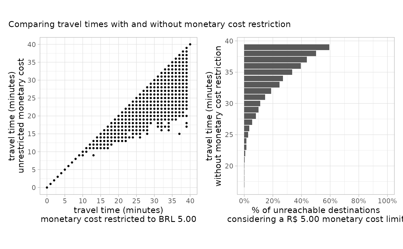

4.2 Calculating accessibility with monetary cost

How many healthcare facilities can one reach within 40 minutes by public transport on a R$ 5.00 budget? Below, compared with an unlimited budget:

# calculate accessibility function
calculate_accessibility <- function(fare, fare_string) {
  access_df <- accessibility(
    r5r_network,
    origins = points,
    destinations = points,
    mode = c("WALK", "TRANSIT"),
    departure_datetime = as.POSIXct(
      "13-05-2019 14:00:00",
      format = "%d-%m-%Y %H:%M:%S"),
    time_window = 1,
    opportunities_colname = "healthcare",
    cutoffs = 40,
    fare_structure = fare_structure,
    max_fare = fare,
    max_trip_duration = 40,
    max_walk_time = 20,
    progress = FALSE)

  access_df$max_fare <- fare_string

  return(access_df)
}

# calculate accessibility, combine results, and convert to SF
access_500 <- calculate_accessibility(fare=5, fare_string="R$ 5.00 budget")
access_unl <- calculate_accessibility(fare=Inf, fare_string="Unlimited budget")

access <- rbind(access_500, access_unl)

# bring geometry
access$geometry <- h3jsr::cell_to_polygon(access$id)
access <- st_as_sf(access)

Mapping both results shows the effect of the budget on accessibility:

# plot accessibility maps
ggplot(data = access) +
  geom_sf(aes(fill = accessibility), color=NA, size = 0.2) +
  scale_fill_distiller(palette = "Spectral") +
  facet_wrap(~max_fare) +
  labs(subtitle = "Effect of monetary cost on accessibility") +
  theme_minimal() +
  theme(legend.position = "bottom",
        axis.text = element_blank())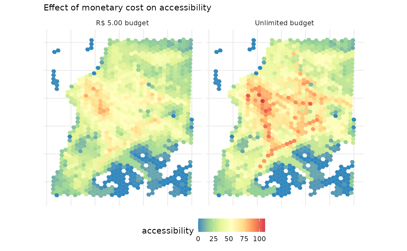

Cleaning up after usage

Stop the network and run Java’s garbage collector to free the memory it used:

r5r::stop_r5(r5r_network)
rJava::.jgc(R.gc = TRUE)

If you have any suggestions or want to report an error, please visit the package GitHub page.

2026-10-10