
Trip planning with detailed_itineraries()
2026-10-10
Source:vignettes/detailed_itineraries.Rmd
detailed_itineraries.RmdAbstract
This vignette shows how to do route planning using thedetailed_itineraries() function in r5r.
1. Introduction
r5r’s routing and accessibility functions are very
fast, but they return only the essential information, and only the
optimal route (minimizing travel time and/or monetary cost). Sometimes,
though, we would like to do more simple route planning analysis and
extract more information for each route. Also, we might be interested in
finding not only the fastest route but some other suboptimal route
alternatives too. This is where the detailed_itineraries()
function comes in. detailed_itineraries() returns, for each
origin/destination pair, a detailed route plan per leg, i.e. a part of
the trip on a single mode, such as walking to the bus stop (R5’s
documentation calls legs ‘segments’). Each leg has its mode, waiting
time, travel time, distance and geometry. The function can also return
suboptimal route alternatives.
obs. Use detailed_itineraries() only if
you need suboptimal alternative routes and/or route geometries. For
route information by trip segment alone, we strongly recommend
expanded_travel_time_matrix().
2. Build routable transport network with
build_network()
We use the Porto Alegre (Brazil) sample data included in
r5r.
# increase Java memory
options(java.parameters = "-Xmx2G")

# load libraries
library(r5r)
library(sf)
library(ggplot2)
library(data.table)

# build a routable transport network with r5r
data_path <- system.file("extdata/poa", package = "r5r")
r5r_network <- build_network(data_path)

# routing inputs
mode <- c('walk', 'transit')
max_trip_duration <- 60 # minutes

# departure time
departure_datetime <- as.POSIXct("13-05-2019 14:00:00",
                                 format = "%d-%m-%Y %H:%M:%S")

# load origin/destination points
poi <- fread(file.path(data_path, "poa_points_of_interest.csv"))
3. Detailed info by trip segment for multiple trip alternatives
To get alternative routes between one origin/destination pair, set
shortest_path = FALSE. With
suboptimal_minutes = 8, r5r also keeps routes
arriving up to 8 minutes after the optimal one.
# set inputs
origins <- poi[10,]
destinations <- poi[12,]
mode <- c("WALK", "TRANSIT")
max_walk_time <- 60
departure_datetime <- as.POSIXct("13-05-2019 14:00:00",
                                 format = "%d-%m-%Y %H:%M:%S")

# calculate detailed itineraries
det <- detailed_itineraries(
  r5r_network,
  origins = origins,
  destinations = destinations,
  mode = mode,
  departure_datetime = departure_datetime,
  max_walk_time = max_walk_time,
  suboptimal_minutes = 8,
  shortest_path = FALSE
  )

head(det)
#> Simple feature collection with 6 features and 16 fields
#> Geometry type: LINESTRING
#> Dimension:     XY
#> Bounding box:  xmin: -51.24094 ymin: -30.05 xmax: -51.19762 ymax: -29.99729
#> Geodetic CRS:  WGS 84
#>            from_id  from_lat  from_lon                          to_id    to_lat
#> 1 farrapos_station -29.99772 -51.19762 praia_de_belas_shopping_center -30.04995
#> 2 farrapos_station -29.99772 -51.19762 praia_de_belas_shopping_center -30.04995
#> 3 farrapos_station -29.99772 -51.19762 praia_de_belas_shopping_center -30.04995
#> 4 farrapos_station -29.99772 -51.19762 praia_de_belas_shopping_center -30.04995
#> 5 farrapos_station -29.99772 -51.19762 praia_de_belas_shopping_center -30.04995
#> 6 farrapos_station -29.99772 -51.19762 praia_de_belas_shopping_center -30.04995
#>      to_lon option departure_time total_duration total_distance segment mode
#> 1 -51.22875      1       14:07:57           35.6           9460       1 WALK
#> 2 -51.22875      1       14:07:57           35.6           9460       2 RAIL
#> 3 -51.22875      1       14:07:57           35.6           9460       3 WALK
#> 4 -51.22875      1       14:07:57           35.6           9460       4  BUS
#> 5 -51.22875      1       14:07:57           35.6           9460       5 WALK
#> 6 -51.22875      2       14:07:57           42.7           8773       1 WALK
#>   segment_duration wait distance  route                       geometry
#> 1              5.1  0.0      174        LINESTRING (-51.1981 -29.99...
#> 2              6.6  2.0     4796 LINHA1 LINESTRING (-51.19763 -29.9...
#> 3              4.0  0.0      256        LINESTRING (-51.22827 -30.0...
#> 4             10.4  4.4     4083    188 LINESTRING (-51.22926 -30.0...
#> 5              3.2  0.0      151        LINESTRING (-51.22949 -30.0...
#> 6              5.1  0.0      174        LINESTRING (-51.1981 -29.99...
The output is an sf data.frame, ready to map.
3.1 Visualize results
street_network_to_sf() extracts the OSM street network
used in routing, to give the map geographic context:
# extract OSM network
street_net <- r5r::street_network_to_sf(r5r_network)

# extract public transport network
transit_net <- r5r::transit_network_to_sf(r5r_network)

# plot
fig <- ggplot() +
        geom_sf(data = street_net$edges, color='gray85') +
        geom_sf(data = subset(det, option <4), aes(color=mode)) +
        facet_wrap(.~option) +
        theme_void()

fig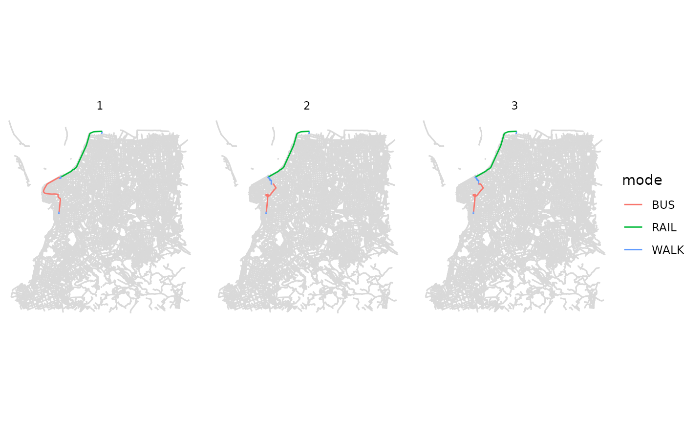
4. Other options
-
All origins to all destinations: by default,
detailed_itineraries()routes the 1st origin to the 1st destination, the 2nd to the 2nd, and so on. Setall_to_all = TRUEto route every origin to every destination. -
No geometry: set
drop_geometry = TRUEto return results without the trip geometry. This makes the function faster.
5. Hack for frequency-based GTFS feeds
detailed_itineraries() does not work with
frequency-based GTFS feeds. The workaround is to convert frequencies to
timetables with the gtfstools
package:
library(gtfstools)

# location of your frequency-based GTFS
freq_gtfs_file <- system.file("extdata/spo/spo.zip", package = "r5r")

# read GTFS data
freq_gtfs <- gtfstools::read_gtfs(freq_gtfs_file)

# convert from frequencies to time tables
stop_times_gtfs <- gtfstools::frequencies_to_stop_times(freq_gtfs)

# save it as a new GTFS.zip file
gtfstools::write_gtfs(gtfs = stop_times_gtfs,
                      path = tempfile(pattern = 'stop_times_gtfs', fileext = '.zip'))
write_gtfs() saves the new feed to the path
you give it (a temporary file above). Put that file in your
data_path, in place of the frequency-based feed, and build
the network.
Cleaning up after usage
Stop the network and run Java’s garbage collector to free the memory it used:
If you have any suggestions or want to report an error, please visit the package GitHub page.